Graphing parametric functions: Survey of methods
Consider a parametric curve given by equations
x = x(t),
y = y(t) for t in some interval
I.
Assume that the functions x(t),
y(t) are
twice differentiable on I. We want to sketch this curve.
Algorithm:
Step 1. Find out what happens at the "ends" of I. If an
endpoint of I is included in I, then substitute this time into
x and y to learn where the path starts or ends. If some
endpoint is not included, find the appropriate one-sided limit of x
and y with respect to t and then interpret this information.
Case "both limits proper": the curve goes toward the point given by the
limits.
Case "both limits improper": the curve goes toward corners depending on
the sign of the infinities in the limits, for instance if
x→−∞
and
y→∞,
then the curve goes toward
the upper left corner. Asymptote can be found using limits
A = lim( y/x),
B = lim( y − Ax),
assuming that they converge.
Case "x→L,
limit of y improper": the curve has a
vertical asymptote at x = L and hugs
this line around its upper or lower end depending on the sign of infinity as
the limit of y.
Case "limit of x improper, y→L":
the curve
has a horizontal asymptote y = L and
hugs this line around its right or left end depending on the sign of
infinity as the limit of x.
Step 2. Find intercepts. The x-intercepts are
given by times t satisfying
y(t) = 0, the
y-intercepts are given by times t satisfying
x(t) = 0. Substitute these times into
x and y to learn spatial coordinates of intercepts.
Step 3. Find  and
and  ,
then find t from the interior of I
satisfying = 0
or = 0. These
are critical times. Substitute them into x and y to find
points where the curve turns.
,
then find t from the interior of I
satisfying = 0
or = 0. These
are critical times. Substitute them into x and y to find
points where the curve turns.
Mark data from Step 1,2, and 3 in the plane. It is recommended to make a note
at each point to indicate at what time the path gets there.
The critical times split I into subintervals. For each subinterval
determine signs of
and ,
then determine signs of the spatial derivative

This is best done using a table. For each subinterval of I that we
obtain, the times from this subinterval give a certain part of the curve and
the increase or decrease of this part as a graph is given by the relevant sign.
It is now possible to connect points in the picture by temporary lines that
fit these trends.
Step 4. Find the second derivatives with respect to time of x
and y and calculate the second spatial derivative
Find times from the interior of I when the numerator or denominator
of this derivative is zero. Substitute these times into x and y
to find points where the curve might change spatial concavity. Mark these
points in the graph.
These times split I into subintervals. For each subinterval
determine signs of the second spatial derivative y′′,
this is best done using a table. For each subinterval of I that we
obtain, the times from this subinterval give a certain part of the curve and
the concavity of this part as a graph is given by the relevant sign of
y′′. We correct the temporary lines to reflect this data.
These are the main steps. If the curve has an end at some endpoint of
I (that is, when this endpoint was included in I or we get
both limits proper in Step 1), it is also a good idea to determine the
appropriate one-sided spatial derivative at that point, it tells us in which
direction the curve should start off. For instance, if it is the left
endpoint t = a of I and we denote
x0 = x(a), then
For more details and another example see
Sketching parametric functions in
Theory - Implicit and parametric functions.
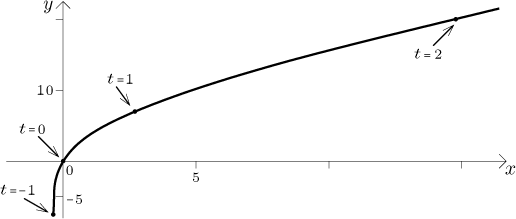
Example: Investigate the parametric curve
x = t⋅et,
y = t3 + 6t,
t ≥ −1.
Solution: The interval I = [−1,∞)
contains its left
endpoint t = −1; substituting into x
and y we get the starting point for the curve
(−1/e,−7). The other endpoint of I is infinity,
so we find

Thus the curve eventually disappears in the upper right corner. The limit of
y/x at infinity is zero, which would suggest a
horizontal asymptote, but the limit for B diverges and thus there is
no asymptote, just the function grows slower and slower (it is pulled more
"to the right" than "up"); we expect that it will be concave at that end.
Intercepts: The y-intercept is given by
x = t⋅et = 0,
which has just one solution, t = 0. This time
gives the point (0,0).
The x-intercept is given by
y = t3 + 6t = 0,
which again gives t = 0 and point
(0,0).
We find (t) = (t + 1)et,
which is zero only for t = −1, the endpoint of
I and therefore the basic time interval does not get split. We also
have (t) = 3t2 + 6,
no zero point here. Thus the graph given by the curve has the same
monotonicity for all times from I. For
t > −1 both (t) and
(t) are positive, hence also
y′(x) is positive and the graph grows.
It remains to find

This derivative does not exist when t = −1 and we ignore
this point as before, and it is zero when t is the cubic root of −4,
which is less than −1 and hence not inside I, we also ignore it. We
see that for t > −1 the second spatial
derivative y′′(x) is always negative, and
therefore the curve is concave down as a graph.
The last piece of data is the one-sided derivative at the beginning of the
curve:
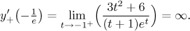
The curve should therefore start vertically up. Since we do not have any
points beyond t = 0, we get a better idea how
things go on by substituting few more times, taking
t = 1 we get the point
(e,7), taking t = 2 we get
the point (2e2,20). We are ready for a
picture.
For another example see
Implicit and parametric
functions in Solved Problems.
Back to Methods Survey - Implicit
and parametric functions