Functions of more variables: Introduction

Functions of more variables are a natural generalization of functions of one variable. A function of one variable is a mapping from one copy of real numbers (typically from some subset) to another copy. We obtain a function of more variables when we replace the starting one-dimensional set with a set of more dimensions.

People usually think of a formula when talking about functions (which is not always possible, but we typically meet them this way), and this also allows for a logical extension: from formulas of the type f (x) = x² we pass to formulas of the type f (w,x, y,z) = (e^w + y)^x⋅sin(x − πz). Notation like f (x, y), f (x, y,z), or f (u,v,w,x, y) is very convenient when we work in a particular setting and know the number of variables, but it is not suitable for general musings, when we work with an unknown number of variables. In such cases it pays to see the situation as if we worked with one variable, just this time we take that variable from a set of vectors. We simply write f ().

In this notation, our work with functions of more variables is often analogous to the case of one variable. Many ideas carry over, just calculations and procedures are sometimes a bit more complicated. All this is markedly easier if we can connect theoretical ideas with geometrical imagination, here some experience with basic objects in more-dimensional space (lines, planes) comes handy.

This is also the main aim of these pages, to show the geometry behind notions, calculations and procedures. We start with the definition of a function of more variables to put our reasoning on firm footing.

Definition.
By a function of more variables we mean any mapping f : D ↦ ℝ, where D = D( f ) is some subset of ℝⁿ.

If D is not explicitely given, then for the domain D( f ) we take the set of all ∈ℝⁿ for which f () makes sense.

Domain

When a function is given by a formula, we determine its domain just like with functions of one variable: We ask what restrictions for the variables arise from that given formula.

Unlike the case of one variable, we need not try to express the resulting set in some standard way (union of intervals), since this is simply not possible in more dimensions; sets come in so many shapes that we are not able to write them down using one basic type of set (or several basic types). Thus it is enough to write the answer as

D( f ) = {∈ℝⁿ; conditions for }.

Conversely, there is one new thing that does not make much sense in one dimension: In more dimensions we can sometimes recognize what kind of object it is.

Example.
We determine D( f ) of the following functions:

a) f (x, y) = x ²sin(x + y):     obviously D( f ) = ℝ².

b) :     D( f ) = {(x, y)∈ℝ²;  x² + y² ≤ 3²},
it is a circle centered at the origin, with radius 3.

c) :     D( f ) = {(x, y,z)∈ℝ³;  x² + y² + z² ≤ 3²},
it is a ball centered at the origin, with radius 3.

d) :     D( f ) = {(x, y)∈ℝ²;  y ≠ x},
it is the plane with a line---the main diagonal---removed (see picture below).

e) :     D( f )={(x, y)∈ℝ²;  y⋅x ≥ 0},
it is the first and third closed quadrant in the plane.

Visualisation of functions (sketching a graph)

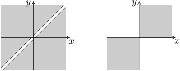
We usually visualise functions of one variable through its graph. Generalizing this notion to more dimensions is easy. In one variable, the graph of a function is a subset of the two-dimensional space determined as the set of all points of the form (x, f (x)) for x∈D( f ). If we take the variable of a function  f () from somewhere in the space ℝⁿ, then we will need one more dimension for the graph, and it is the set of all points of the type (x₁,x₂,...,x_n, f ())∈ℝⁿ⁺¹, where  = (x₁,...,x_n).

When n ≥ 2 we therefore need at least three dimensions for the graph, meaning that we jump out of our paper. We see that such a graph actually cannot be drawn. Still it is worthwile to think about graphs and work with the idea: On a "horizontal" representation of domain (precise or symbolic) we find the position of a certain multi-dimensional variable, and we draw a dot of the graph above it at elevation corresponding to the function value at the given variable.

If we do this at all points of the domain, the corresponding dots create a certain object that we can imagine to be a sort of wavy surface. This is what in fact happens with functions of two variables, a typical graph of such a function is some thin (essentially two-dimensional) object inside a three-dimensional space. With a bit of luck we can get a very suggestive picture of it using shading and similar methods. For instance, the graph of a constant function f (x,y) = c is the horizontal plane floating above the basic axes x,y at the appropriate elevation c.

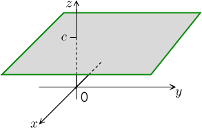
We like to work with functions of two variables precisely because we can usually sketch them. Experience should suggest that there also are functions of two variables whose graphs are not that nice, it could be just some scattered bunch of points in ℝ³, but we do not expect to find such functions in applications.

If we have three or more variables, then we cannot even sketch a likeness of a graph, four-dimensional space is beyond our imagination. People then employ other means that would allow us to get a visual feeling for a function's behaviour. We will show here the most popular approaches.

It should be noted that these methods are also useful for the case n = 2, because they help us to deduce how such graphs actually look like, to draw faithful sketches. Since we can really draw pictures for functions of two variables, we will actually see how those methods work. In this way we get some insight into the new notions that will hopefully extend to higher dimensions, where we cannot really imagine how things look.

There are also other methods for obtaining sketches of functions of two variables, notably using appropriate programs (Maple, Mathematica and such), which is convenient and nice. However, it is useful to understand things well, after all, those programs sometimes fail and then we have to rely on the good old brain and our knowledge.

Level sets.

This is one of the most powerful visualisation methods, but this notion also has a wider use, for instance when investigating objects that were defined implicitly.

Definition.
Let f: D( f ) ↦ ℝ be a function, where D( f ) ⊆ ℝⁿ. For c∈ℝ we define the corresponding level sets

L_c = {∈D( f );  f () = c}.

How does it work? First we slice the graph at level c (we ask where the values of the function are equal to c) and then we check for which values of variable we get there, that is, we project that cut into the domain. If we imagine the graph to be a tract of land, then level sets are places given by their geographical coordinates (that is, places on a map) on which the elevation is precisely c. In other words, level sets are analogous to contours on a map. An experienced tourist can guess the shape of land just by looking at contours, similarly we can deduce a lot of useful information from level sets.

When working with functions of two variables, we traditionally say level curves instead of sets, and with three variables we often say level surfaces.

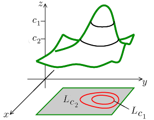
From the definition we see that L_c lies in D( f ), so just n dimensions are enough to show level sets, an advantage compared to graphs. It is a handy way of analysing functions of three variables. For example, if we have a function T(x,y,z) describing temperature at various places in a certain room, then for temperature c we see level sets (surfaces) L_c as "clouds" showing us where in the room that temperature is. These clouds are three-dimensional, we can use a perspective drawing to show them in 2D (on paper). Comparing such sketches for varying values of c we get a rather good understanding of behaviour of temperature, it is also possible to connect these pictures into an animation etc. The picture below shows two possible temperature "snaps" of a classroom in February when it is being heated by three students sweating an exam.

Cuts (slices).

Slices are a simple but very powerful tool for exploring more-dimensional situations. However, they will be really simple for us only if we understand well the interplay between formulas and geometric meaning. The basic idea is that we create a two-dimensional "slice" of a multi-dimensinal situation by cutting it with a plane. Such a slice can be (hopefully) explored using tools for investigating (graphs of) functions of one variable.

Assume we are in a situation when the variables are taken from the world of ℝⁿ, we can imagine it symbolically as a horizontal object in our picture. We choose some starting point and consider a straight line p in ℝⁿ passing through this point in direction . Points of this line are given (if we assume uniform movement) by the parametric equation  =  + t, we can imagine that it is a description of a journey we take through the domain D( f ). At time t we are at a certain point from D( f ) and we see the function value f (+t) corresponding to this point. We thus obtain a mapping t ↦ f (+t) describing the shape of the graph that we "see" above us while moving along the line p. This line therefore determined a slice that we obtain as an intersection of the graph of f and "vertical" plane erected over p.

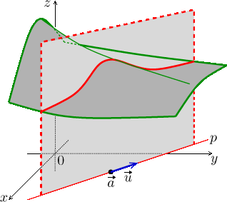
The shape of this slice is obviously related to the function φ(t) = f (+t), which is a function of one variable and we can readily investigate it. Unfortunately this relationship is not as simple as we would hope, that is, that drawing the graph of the function φ(t) would already show us the shape of that slice. The problem lies in scale. In our two-dimensional picture of the slice, the mark for "1" (position at time t = 1) is at the place  + , which does not necessarily need to be at the distance 1 from the point in our original many-dimensional picture of the graph of f. The amount of distortion obviously depends on the size of the directional vector , which should not surprise: The faster we go, the more the landscape around gets subjectively distorted (it get "squeezed", we pass things quicker). Therefore we prefer directional vectors of magnitude one (unless the situation we are in prevents us, for instance when we are working with some applications), then the geometric information agrees. We will encounter these considerations again in the section on derivatives.

Example
Consider the function

We will investigate the slice through its graph that we obtain by cutting it with the plane above the line (x,y) = (2,3) + t(−1,1). Interpretation: Function f indicates elevation, we stand at a place with GPS coordinates (2,3) and start off in the direction (−1,1). As we walk, we are interested in raise and fall of the land.

The description of the line yields formulas x = 2 − t, y = 3 + t, substituting them into the function f gives the auxiliary function

The last expression shows that the graph of the function φ is shaped like a hill whose summit (maximum) is at time t = 1. It is not the precise shape of the slice through the graph of the function f, because |||| = ||(−1,1)|| is equal to square root of two, it is not a unit vector. The real shape is therefore - compared to the graph of φ - shrinked in horizontal direction, but that does not change it main outline. We can thus conclude that the corresponding cut through the graph of f is shaped like a hill whose highest point is at the point corresponding to time t = 1, that is, the point (1,4).

We remark that this need not necessarily mean that the graph of the function f as such has a hill there. To see a situation of this sort, look at the picture above. The graph there is not exactly like our f, but the situation fits quite well: We cut through a sloping landscape and get a hill on the slice. The picture even has the point , vector and line p at the right places and the shape of the slice is essentially correct.

We also remark that if we wanted to see the precise shape of the slice, or if we wanted to work analytically with its geometry, we would have to consider the directional vector

The calculations are then analogous, just a bit less pleasant.

We prefer to work with lines parallel to coordinate axes, since then we get information that is easy to handle both graphically and analytically (we see the influence of individual variables). For instance, if we are in ℝ³ at the point (x₀, y₀,z₀) and we want to move in the direction of the y-axis, then we obtain the line t ↦ (x₀, y₀ + tu,z₀). In other words, the variables that we do not care about are left constant and we change only one. This is a very simple process. Since we prefer directional vectors of magnitude 1, we typically work with pleasant lines of the form t ↦ (x₀ + t, y₀,z₀), t ↦ (x₀, y₀ + t,z₀) etc. This means that we fix values of most of variables and one is left to change in the usual manner, which is also reflected in the notation: We need not introduce t, just investigate lines such as x ↦ (x, y₀,z₀), y ↦ (x₀, y,z₀) etc.

This idea can be generalized as follows: We fix a certain number of variables and move with the others, which allows us to lower the number of dimensions we work with, depending on what we are currently interested in. Consider a function T(x, y,z) of three variables, for instance a description of temperature in various places of a lecture room, and a certain point  = (x₀, y₀,z₀).

If we fix values y = y₀ and z = z₀, we get a one-dimensional object, that is, a line leading as from the point in the direction of the x-axis, and as we go along, we see the temperatures. It is a one-dimensional situation x ↦ T(x, y₀,z₀) that we easily investigate and draw.

If we fix only the variable z = z₀, then we have two degrees of freedom, that is, we move on the (horizontal) plane passing through the point perpendicular to the z-axis. Thus we obtain a function of two variables (x, y) ↦ T(x, y,z₀) whose graph we can (with a bit of luck) visualize using a perspective drawing (with shading, for instance).

In this way we get another tool for investigating functions. Still, most often we work with movement along a line and one-dimensional situations.

Standard shapes.

When working with functions of one variable, we often think of its graph as an analytical object in the plane given by the equation y = f (x), and we can recognize many of these objects. For instance, the graph of the function f (x) = 1 − 2x is the object described by the equation y = 1 − 2x, that is, 2x + y = 1, and we know that this determines a line. This trick sometimes works rather well also with functions of more variables.

For functions of n variables we obtain an object in ℝⁿ⁺¹ determined by the equation y = f (). We can hope to recognize such an object. For instance, the function f (x, y) = 2x + y − 5 leads to the equation 2x + y − z = 5, which defines a plane in ℝ³.

Sometimes we have to reorganize the equation we obtain, but then we have to be careful about changing the resulting set. This is actually nothing new, we had to be careful already when working with functions of one variable. For instance, we know how the graph of the function f (x) =  looks like. If we rewrite the equation y =  as x = y², we immediately recognize this object as parabola, just the roles of variables are reversed. Therefore this is a parabola that goes to the right, above and below the x-axis. However, the graph of our function f (x) =  is only the top half of this object.

Such change in size of a set (getting larger or smaller) happens when we use some non-equivalent steps when rewriting our equation, the squaring that we used above is one popular case. Experience should suggest when it is time to pay extra attention.

In order to be sussessful in recognizing shapes we need to know basic geometric objects. The most popular are flat objects (lines, planes) and objects given by quadratic equations, which in two dimensions means the well-known family of conic sections (parabola, circle and, more generally, an ellipse), in more dimensions we get a richer family. It seem clear that one would have to be really lucky to hit one of the few known equations when choosing from infinitely many functions, but it actually happens more often than one would expect from purely probabilistic standpoint. And when it does happen, it is very helpful.

Example.
Here we will showcase our methods on the function

Domain: D( f ) = {(x, y)∈ℝ;  x² + y² ≤ 3²}.
It is the circle of radius 3 with center (0,0). The graph will be above this circle as obviously f (x, y) ≥ 0.

We start with level curves. We see right from the definition of the function that its values are in the range between 0 and 3, the corresponding level curves will therefore be interesting, the other ones are empty. So how does a level curve L_c look like for c∈[0,3]?

It is the set given by the relation f (x, y) = c that is, x² + y² = 9 - c², this specifies the circle of radius lying in the domain. For larger c (larger values of the function) these circles get smaller, closer to the origin, and conversely, for c = 0 we get for the level curve the circle of radius 3, the boundary of the domain.

Conclusion: The function is equal to zero on the edge of the domain, it is largest at its center, hills look this way. In the picture we see level curves in red in the domain, the corresponding values are indicated using dashed lines on the graph.

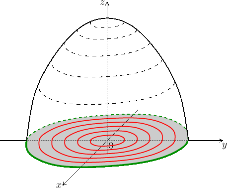
Because the level curves are rotationally symmetric with respect to the origin (they are circles), we can deduce that the graph is also symmetric with respect to rotation about the z-axis.

Now we look at slices. If we fix x = 0, we are in effect asking how the graph looks like above the y-axis. We get

this has an upper half-circle as its graph. For other fixed x = a, the graphs of slices are smaller half-circles

So this is how cuts using vertical planes parallel to the y-axis look like.

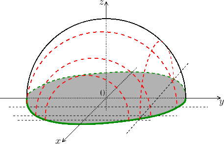
It also works symmetrically, so vertical slices through the graph of f parallel to the x-axis are upper half-circles as well. It would seem that this graph is not just any hill, but a hill of spherical shape.

We try to confirm this guess by recognizing the shape. The graph of f is given by the equation

which we readily rewrite as x² + y² + z² = 3² and we have the equation of sphere. Obviously the whole sphere cannot be the graph of our function (because it would offer two values for one point (x, y)), but some subset of it. Since D( f ) is the circle of radius 3 in the xy-plane, the graph must cover the whole expanse of that sphere, and from f (x, y) ≥ 0 it follows that we should look at its upper half, which is something that we already guessed from level curves and cuts.

Conclusion: The graph of f is the upper half-sphere (a dome).

Example.
Now we look at the function

f (x, y) = x² + y².

D( f ) = ℝ².

Level curves: x² + y² = c, these are circles whose radii are increasing with larger values of the function. So the farther we are from the origin, the bigger the function, this looks like a pit. Since all level curves are invariant with respect to rotation (they look the same after rotating them about the vertical axis), the graph will also be like that.

Slices: If we choose x = 0, we get f (0, y) = y², this is parabola. For other fixed x we get parabolas shifted up f (x₀, y) = x₀² + y², the shift grows larger the further we are from the origin. The verteces of these parabolas are themselves on a parabola. This is true also symmetrically, when we fix y.

When we put this together our observation about rotational symmetry, the conclusion is clear. The graph is a paraboloid, that is, a rotated parabola.

Example.
Now we look at the function

f (x, y) = x² − y².

D( f ) = ℝ².

Level curves: x² − y² = c, these are hyperbolas of growing radii.

Slices: If we choose x = 0, we get f (0, y) = −y², the graph is a parabola oriented downward. For other x we get upside-down parabolas shifted up, f (x₀, y) = x₀² − y², the shift growing as we get further from the origin. Verteces of these parabolas lie on a parabola oriented up.

If we choose y = 0, we get f (x,0) = x², the graph is a parabola. For other y we get parabolas shifted down, f (x, y₀) = x² − y₀², the shift growing as we get further from the origin. Verteces of these parabolas lie on a down-oriented parabola.

Supplemental methods: there is no symmetry of rotation, the equation z = x² − y² is not universally known. So not much help here, we have to make do with slices.

Conclusion: It is an interesting graph worth drawing.

Functions of more variables: Derivative
Back to Extra - Functions of more variables