Functions of more variables: Integral

We start with an outline of definite integral for functions of one variable that is not formally correct but conveys the right idea. The expression

Now we extend this idea to functions of more variables. If we have some set Ω in ℝⁿ and a function f on it, then we also can "add" values. However, this time we do not work with flat rectangles but more dimensional "columns". In case when Ω is in ℝ², that is, we have a function of two variables, then over every point we can imagine a superthin cylinder of height f () and with base dA, where dA is now an infinitely small piece of a plane, it is a plane differential.

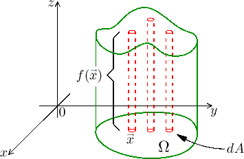
If we "add" their volumes -- which are obviously f ()⋅dA, -- using the symbolic operator ∫, we obtain

This is called the double integral. Its meaning is intuitively clear, it is the volume of the solid whose base is Ω and its top part coincides with the graph of the function f. Just like in case of one variable, also here the volumes are subtracted when f () < 0, so it is a "mathematical volume". It should be noted that the idea of columns is the important part, not the particular cylidrical shape. For instance, later we will find it useful to work with columns with square bases.

We readily generalize this idea of double integral to functions of even more variables, for instance

is the four-dimensional size of the object "under" the graph of a function f of three variables. Since such a function takes its variable from the space ℝ³, the "bases" of the "columns" we add are three-dimensional, which explains the notation dV, it is the volume differential. This is called a triple integral, in general we talk of multiple integrals. Obviously we have trouble visualizing, say, a seven-dimensional column with a six-dimensional base, but that should not be a big problem as the basic idea remains. We are simply "adding" values of the function at all points from the given set Ω.

Remark.
Sidenote on terminology: In mathematical analysis, "region" is a special term describing a set that is connected and open. Unfortunately, when it comes to integration, people traditionally use the word region for the set over which we integrate, regardless of its properties. While we usually do integrate over connected sets, they are rarely open, in fact, in most cases the set Ω is closed. This is unfortunate, but the word "region" somehow fits with the whole integration picture and pretty much everybody uses it. I tried to use "set" instead so that this text is precise, but somehow "region" sneaked in anyway, so I left it here. Please be aware that in this particular chapter region does not mean a mathematical region, in particular it need not be open, it is just another word for a set.

The main idea of a more-dimensional integral seems clear, but it is not obvious how one would go about actually calculating such an integral. We will try our favourite trick and introduce slices, which turns the problem into a one-dimensional affair. We will arrive at cuts in axial directions by organizing "columns" smartly.

As usual we first look at functions of two variables. There we will utilize the idea that we add superthin rectangular boxes whose bases dA are infinitely small squares dx×dy. We choose a basic direction, say, along the y-axis. Just like with derivatives, we fix x to some number x = x₀ and we check on all boxes that correspond to this value. They stand next to each other, they share common width dx, and therefore they create a sort of board with an irregular upper edge (it is given by the function f ). The volume of this board is obtained by multiplying its side area by the thickness dx.

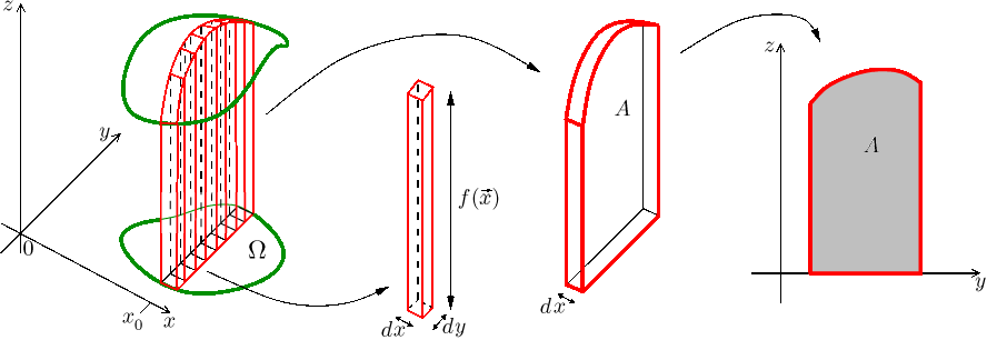
That side area, the slice through the graph of f, can be easily determined; it is the area under the graph of the function y ↦  f (x₀, y), in other words it is the classical integral of a function of one variable.

We will now try it again, but with some mathematics. If we choose x = x₀, then we are interested in the set of all points (x₀, y), that are in the given set Ω. In other words, we consider a straight line going through the domain in the direction of the y-axis, just like in previous sections, and we are interested in its intersection with the set Ω. This intersection can be very wild, but for simplicity we restrict ourselves to sets Ω shaped in such a way that all such cuts through it (for all choices of x) are either empty (we do not care about those), or have the form of a segment with certain endpoints given by c(x) and d(x).

So for a chosen x₀ we are interested in points (x₀, y) for values y satisfying c(x₀) ≤ y ≤ d(x₀). For those y we have a function (of one variable) y ↦  f (x₀, y), which we can---with a bit of luck---integrate. In this way we obtain a certain number

which is the two-dimensional area of the slice through the solid under the graph of f.

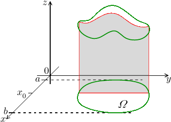
To make things practical we just pretend that x is a constant and integrate with respect to y. It is the same idea as with partial differentiation, so it should not cause much trouble. Note that we obtain a number that depends on the choice of x, but the variable y gets used up during integration.

which is the volume of the slice as a three-dimensional object that we obtained above by organizing the thin rectangular columns.

We get other slices by changing the fixed value x. To include the whole volume of the solid, we need to "add" volumes of individual slices, which we will obviously do by integration using x. It all nicely fits together, as we already observed that volumes of slices depend exactly on the choice of x. The least value a and the largest value b for x are determined by which slices through Ω are non-empty. We get the formula

In order for this whole thing to work, the set Ω must be shaped in such a way that we are able to find the functions c(x), d(x) for endpoints of slices and limits a, b for x. In other words, we are talking here about regions Ω squeezed between two curves over an interval:

Ω = {(x, y)∈ℝ²;   a ≤ x ≤ b   and   c(x) ≤ y ≤ d(x)   for all   x∈I}.

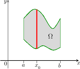
Then

Such a reworking of a double integral is called a repeated integral.

It is good to learn how to rewrite such an integral just using a picture of Ω, without referring to the graph of the function (which needs an extra dimension). We want to use a double integral to pass through all points of the set Ω. We decided to go through them via segments parallel to the y-axis, in our picture above it means vertical slices. The inner integral runs over a typical slice whose endpoints obviously depend on the location of this particular slice, that is, on x. Using the outside integral we then run through all the slices by changing x.

As one can expect, it is not necessary to start cutting in the y-direction. The set Ω could be oriented the other way,

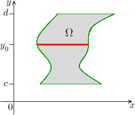
that is, the set could be of the form

Ω = {(x, y)∈ℝ²;   c ≤ y ≤ d   and   a(y) ≤ x ≤ b(y)   for all   x∈I}.

This is the second possible expression for a double integral.

Some sets fit with both specifications, then we can choose in which direction to cut.

Example.
We will integrate the function f (x, y) = y⋅e^x over the two-dimensional interval [0,1]×[1,3], that is, the set

Ω = {(x, y)∈ℝ²;   0 ≤ x ≤ 1   and   1 ≤ y ≤ 3}.

We have a choice which variable to use for the first integration, because in a rectangle slicing in both directions works. If we want to integrate with y first, that is, to fix x and slice in the y-direction, then y changes between 1 and 3 regardless of the slice's position.

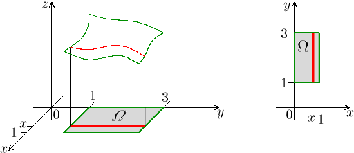
The picture on the left is just symbolic, the graph most likely looks differently, it is there only to remind us of the general situation. We are more interested in the picture on the right, we should be able to deduce all necessary information from it.

For the integral over one slice we get

where x is taken as a constant. Then also e^x is a constant and we have

As we expected, the variable y disappeared and the "area" of the slice depends only on its position given by the value of x. Now we "add" these slices (integrals) using x, we get

Some observations:

1) It is not always possible to factor out the variable we do not use. This should not be a problem, we just pretend that some terms are constants and work with them as usual. Thus we could have evaluated the first integral also this way,

Since there are two variables in the function, to be on the safe side we reminded ourselves where to substitute the limits.

2) We do not have to evaluate the slices separately, it is possible to first set up the whole double integral and then evaluate it. We always do it in the same way, first we evaluate the integral that is inside and then the one on the outside, then perhaps the one that is even more outside and so on. The integration limits and differentials are paired in a nested way: the outer integral belongs with the differential on the outside, the second integral from the left belongs with the second differential from the right etc. It is not permitted to mix them up. Since the evaluation means that we integrate and again and again, integrals of this form are called "repeated integrals".

3) When setting up an integral, it is possible to start from the outside. We will show it in the next example below.

To get some practice with setting up the integral from the inside (that is, from the slices) we will try horizontal slicing, these are also possible here.

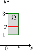
We can deduce from the picture that on every slice x changes between 0 and 1, we get

where y is taken as a constant. We then "add" these integrals using y, we get

We say that we set up a corresponding double integral for the given integral. We evaluate from inside, to emphasise this point we use parentheses to indicate the order, normally we do not do this.

When substituting into the inner integral we reminded ourselves what the working variable was at the time, that is, where should we substitute the integrating limits.

Summary: When we are given a double integral

we rewrite it as a repeated integral

(or in the other order). When evaluating, we start with calculating the inner integral

which gives raise to a function of variable x. Then we evaluate the outer integral

Now compare the two rewritten forms of the integral from the above example:

It looks as if we just switched the integrals and the corresponding differentials "d". However, it is this simple only when integrating over rectangles. In other cases, the so-called "change of order of integration" is a bit more complicated.

Example.
We will integrate the function f (x, y) = e ^x2 over the finite region Ω determined by the curves y = 2x, x = 1, and y = 0. This time we will show how to set up a repeated integral from the outside.

It always pays off to draw a picture of the region of integration, it is a triangle with vertices (0,0), (1,0) and (1,2). Vertical slicing (in the direction of the y-axis) will surely work.

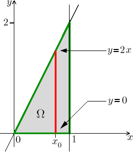
We see that we obtain a meaningful slice only by choosing x between 0 and 1, which tells us how the outside integral should go. The resulting repeated integral will therefore be of the form

On one particular slice, the variable y moves between the values y = 0 a y = 2x. After all, this corresponds to the formal description of the set in the form

Ω = {(x, y)∈ℝ²;   0 ≤ x ≤ 1   and   1 ≤ y ≤ 2x}.

Now it is time to try horizontal slices.

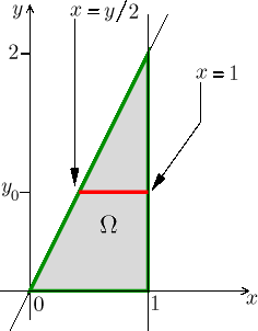
Location of a particular slice is determined by choosing y from the range between 0 throught 2, this makes obvious how the outside integral will go. The slice (on which x is the working variable) is a segment with its right end at the level x = 1, the left end lies on the curve given by the formula y = 2x and we need to know about x. We therefore see that when moving along such a slice, x goes from y/2 to 1. We obtain

We start with the inside integral

And we run into trouble right away, the antiderivative to e ^x2 cannot be expressed by an elementary algebraic formula, so this is the end of the road.

We see that our choice of the slicing direction, that is, our choice of the order of integration can have a big impact on the evaluation that follows. In less extreme cases it may influence the level of complexity of our calculations.

Although one of our attempts did not work out, it was still a useful exercise. Both ways of rewriting the integral were entirely correct and knowing how to set up an integral in this way is a basic knowledge. We also saw that when we changed the order of integration, the integrating limits did change.

This is typical, when changing the order, we have to rework the limits for integrals. Sometimes we are given a repeated integral and we are supposed to change the order of integration (one reason may be that we are not able to evaluate the integral as given). In such a case we first need to reconstruct the shape of the integrating region Ω using the known integrating limits (some sort of a reverse engineering), then we apply slices in the other direction to this region.

The two reworkings of the integral above show one more thing that beginners have to be careful about. When a repeated integral is set up properly, the following must be true (among other things): The outer integral has only numbers for its limits. The inner integral can take numbers or expressions with a variable for its limits, but this variable must be the outer one, the one that is last in the list of differentials.

An inquisitive reader has surely already thought of the fact that not all sets Ω fall into the two types we covered. In such a case it is usually possible to split this region into subregions that are of the right type, then we set up an integral for each of them. This is possible thanks to the linearity of integral with respect to the integrating region. Precise statement of what we mean is a bit more complicated in more dimensions, but roughly speaking is goes as follows:

Consider a region Ω that we split into subregions Ω₁,...,Ω_m in the following sense: Ω = Ω₁∪⋅⋅⋅∪ Ω_m and subregions Ω_i can mutually intersect only over their borders, in other words, their mutual intersections have zero area. Then

Example.
Let Ω be a region between y = x² + 1 and the x-axis above [0,1]. We want to find

First we draw Ω and analyze our slicing options.

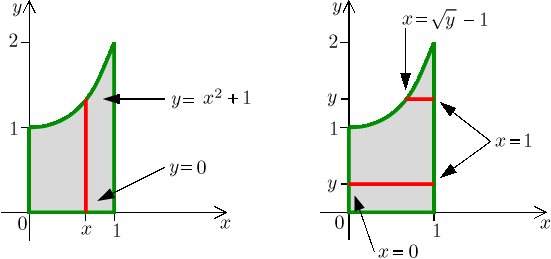
The shape of this set just calls for vertical slicing, where we first integrate with respect to y. Indeed, we see that if we tried slicing in the x-direction, then we would not get a universal formula for left endpoints of slices.

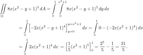
So we have the inner integral with variable y. We note that when integrating the function 8x(x² − y + 1)³ by y, then 8x is actually a constant and we can factor it out of the integral. When integrating the expression (x² − y + 1)³ with respect to y, then also the term x² + 1 is treated as a constant, so in fact we integrate an expression of the form (−y + a)³. An experienced integrator works that out right away, those more careful can try a suitable substitution. It is crucial to differentiate by the right variable when setting up the substitution---it is obviously the one we integrate with right now.

We get

What if for some reason we do want slices in the x-direction? While all the right endpoints of slices are given by the same formula x = 1, the left endpoints are given by x = 0 for y∈[0,1] and by a different formula for y∈[1,2], there x starts on the curve y = x² + 1, Therefore the starting value for x is . We handle this complication easily by decomposing the region Ω into its upper and lower part, each of which has the right shape. In other words, we set up two integrals.

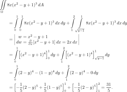
Whew, we got the same answer. I was apprehensive the whole time, fearing that I might be forced to search for a mistake in calculations.

And that's about it.

Remark.
If you are curious how to work out a triple integral

In this case Ω is a three-dimensional object. We need to add values of f at all points of this set, to do so we need to organize them using slicing.

If we fix one variable, say, x, then we obtain a cut through this object that is perpendicular to the x-axis, but only for values of x from some range a through b. In this way we get the first level of decomposition

Now we need to integrate over a typical slice, but that is a two-dimensional object in directions y and z, its particular shape depends on the choice of x. If we are lucky, it is a region of reasonable shape, meaning one of the two types we covered above.

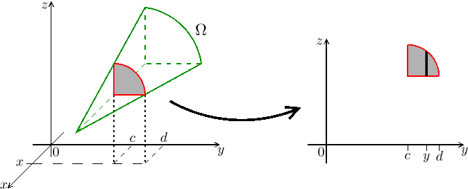
We know how to do double integrals, for instance, with a bit of luck the slices (one-dimensional) in the y-direction might work. Those make sense only for y taken between certain values c(x) and d(x), as the shape of the two-dimensional slice depends on x. The variable z then runs over a segment whose ends depend both on the shape of the particular two-dimensional slice (that is, on x) and on the choice of segment, that is, on y. In this way we arrive at

Of course, we do not know in general that exactly this particular order od slicing will work, there are six possible orders and depending on the shape of Ω at least one should do.

It is quite obvious that in order to be able to set up such an integral one needs a good spacial imagination and mastery of analytical treatment of geometrical shapes.

Remark.
What use can such "adding of values" be? Here is one example.

When we have n numbers x₁,x₂,...,x_n, we find their average using the formula

we need to add them for it.

If we have a function f on some interval [a,b], we find its average value there using the formula

If we have a function f (x, y) on a region Ω, we find its average over this set by the formula

And if you have a function T(x, y,z) describing the temperature at different points of a certain room, in order to determine the average temperature there you would have to "add" all values of T using a triple integral of T over that room (and then divide by its volume).

Back to Extra - Functions of more variables