Derivative of parametric functions

Consider a parametric curve given by
x = f (t),
y = g(t)   for t from an interval I, where f and g are continuous functions.

Consider also a point (x₀,y₀) that lies on this curve, therefore x₀ = f (t₀) and y₀ = g(t₀) for some particular time t₀. With a bit of luck, there is a neighborhood of this point on which the curve can be described using a function y = y(x). In the section Parametric functions in Functions - Theory we have a theorem which has a sufficient condition for this happening. This condition reads f ′(t₀) ≠ 0.

This condition means that f is either increasing or decreasing at t₀, therefore at that time the curve moves left or right as it passes through the given point. The theorem asserts that we can describe the curve using a function there. We can imagine that the function f is actually 1-1 around the given time, therefore we can find its inverse t = f₋₁(x) and use it to eliminate t from the equations. We get

y(x) = g( f₋₁(x)),

see Parametric functions in Functions - Theory. If we assume that f and g are differentiable at t₀, the whole function on the right is differentiable, therefore also y(x) and we even have a formula for the derivative. It gets even more interesting if we use the formula for the derivative of the inverse function (see Derivative and operations in Theory - Introduction). We get the following theorem:

Theorem.
Consider a parametric curve given by
x = f (t),
y = g(t)   for t from any interval I.
Assume that f and g are differentiable at some t₀ from the interior of I and that f ′(t₀) ≠ 0. Then there is some neighborhood of t₀ on which the corresponding part of the curve can be expressed using a function y = y(x).
Moreover, this function is differentiable at x₀ = f (t₀) and we have

We used functions f and g instead of writing the traditional x = x(t), y = y(t) for the description of the coordinates. If we went the traditional way, we would have things like t = x₋₁(x), where the first x is a function and the second one is the variable, quite confusing for a beginner. But now that we have an answer, it might be interesting to rewrite this in the traditional terms, recall that the dot denotes derivative by time.

It gets even more interesting when we use the Leibniz notation.

Now it looks like ordinary cancelling, so the Leibniz notation again makes things look natural.

Note the interplay between time and spatial reasoning. We can view this curve as an ordinary object in the plane, or we can view it as a record of some movement in time. When we want derivative with respect to the x-coordinate at some point in space, the formula relates it to an expression that features time derivatives, quite naturally we also substitute time, namely exactly the time at which we reach the given point. This is quite natural, but it may be confusing if one is not careful enough. When investigating parametric curves, one needs to keep track what is spatial and what is time-relevant. For more insight into this rule see the next section.

Having the formula for the first derivative, we can differentiate it once more to get the following.

Theorem.
Consider a parametric curve as in the previous theorem with all the properties listed there. Assume moreover that f and g are twice differentiable at the t₀. Then the function y = y(x) is also twice differentiable at x₀ = f (t₀) and we have

Using the traditional notation for a parametric curve we get

How did we get this result?

Then we just substitute in x₀, use f₋₁(x₀) = t₀ and we are done.

Example: Consider the parametric curve
x = t⋅e^t,
y = t³ + 6t   for t ≥ −1.
Prove that on a neighborhood of (e,7) we can express this curve using a function and find its derivative.

Solution: The time corresponding to the given point is t₀ = 1. We see that (1) = 2e, which is not zero and therefore the existence of a function y = y(x) on a neighborhood of (e,7) is proved.

By the above theorem we also have

Changing parametric curves into functions

We know how to differentiate a local spatial description, now we return to the problem of decomposing a given curve into parts that can be expressed by functions. We know that changing parametric equations into a function is done by elimination, for which we need the function x(t) to be 1-1. One simple way to recognize intervals of injectivity is to use derivatives.

Assume that we can split the interval I into subintervals on each of which the derivative (t) exists and is not zero and has the same sign. Then on each of these intervals the derivative must be either positive or negative, therefore x must be 1-1 there (see Derivative and monotonicity in Theory - MVT). Thus the pieces of the curve that correspond to time taken from each of these component intervals are exactly the pieces that can be (at least theoretically) expressed as functions.

Note that the sign of the derivative (t) also carries another information, useful when investigating the given curve. When (t) > 0, then the curve goes to the right; when (t) < 0, then the curve goes to the left. But this gets us close to the topic of sketching a given curve, which is covered in the next section.

For a review and an example of parametric curves see Parametric functions in Methods Survey, there is also an example in Solved Problems - Parametric functions.

Bug's Life

Now we return to where we started. The whole point of this section has been to forget about moving around and reduce parametric curves to pictures and functions. We were quite successful, in fact in the next section we learn how to sketch parametric curves. But now we leave this topic and ask what other information can be deduced from a parametric curve.

Given that a parametric curve is a record of a movement, one natural question is about the instantaneous speed at any given point. We have a formula for that.

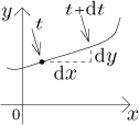
How do we get it? Assume that a bug is at time t at some place and then moves by time dt. In space this means movement by dx and dy, but since x and y are functions of t, we get transformation formulas

dx = ⋅dt,     dy = ⋅dt.

(See Leibniz notation in Theory - Introduction.) Since we moved by an infinitely short time, the curve did not have time to bend and we can think of it as a straight line.

Thus the change ds in position s can be calculated using the Pythagorean rule:

When we divide by dt, we get the desired equality, since speed is exactly the time derivative of position.

We can learn more, for instance we can calculate the length of the path taken, but that requires integration; we refer to Curve length in Integrals - Theory - Applications. In Area in Integrals - Theory - Applications you find how to calculate the area of the region given by a parametric curve, there are also some tidbits about the center of gravity.

Sketching parametric functions
Back to Theory - Implicit and parametric functions