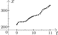
Imagine the following situation. We drive somewhere and for some reason we decide to keep track of the distance that we have travelled. Probably the easiest way to do this is to mark the numbers appearing on our odometer. For instance, assume that when we start, it shows 213. This means that if we want to know how much we travelled at any given moment, we simply subtract 213 from the number that has just appeared on the dashboard.
To complete the setup, we will assume that we start at 9am and arrive at
11am. To make things more proper, we will convert time to the decimal system,
so for instance
So we drive and we keep writing down couples "time - number on odometer at this time", at the end we end up with a chart of many such couples. The more often we do these measurements, the more precise our chart will be, the more information about our trip we will have. One handy way of visualizing this set of data is to put them into a graph, t is for time and x for the number:

Of course, one could use some machinery, say, a computer that would automatically jot down this data, in this way we can obtain couples "time - miles" with frequency of thousands per second. However, the resulting chart would still be "discrete" and with "holes", that is, we would have data only for distinct times. However, if we want to apply the power of mathematics to this situation, we would need to have a measurement for every possible time between 9 and 11 (which is infinitely many times and thus impossible to do in reality). We therefore need to do a little abstraction here and imagine that it is possible, that we can really somehow get an infinite chart of couples "time - number" that covers all times between 9 and 11. For instance, we can imagine that we keep increasing the precision of measurement and keep "filling holes" in the graph.
Thus we get a graph with a really untinterrupted line.
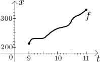
This abstract set of infinitely many measurements is what we call a
function, some sort of a prescription that takes an argument (time in this
case) and hands out a related number. Since as the argument
of this function we use time, we take arguments from the set of real numbers.
The values are also real, so this is a real function; we will call it
f. The notation
We arrived at the notion of a function, now we will review some notions
connected with it. We start with domain, the set of arguments for
which the function makes sense (that is, numbers t that can be put
into the function). Here we have no information about what happened before 9
and after 11 (we will have to agree on how to interpret numbers like 150 and
−3, but this is no problem, we can arrange days one after another and number
time successively, so for instance −3 is 9pm of the previous day, while
D( f ) = Df = dom( f ) = [9,11].
What are the values of function f ? Since the odometer started with 213 and ended with 330, our measurements cannot yield numbers larger than 330 and smaller than 213 (we are assuming here that we did not monkey around with the odometer). One can also argue that all numbers between 213 and 330 must appear in our chart, since the car cannot jump from one position to another without going through all intermediate positions. Thus we guess that the range of f is the closed interval between 213 and 330, which we can write like this (again here we prefer the first notation):
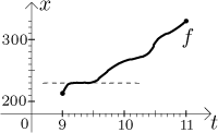
Is this function 1-1? In
practice it is usually easier to ask whether the function fails to be 1-1,
which can be stated as follows: Is it possible that two distinct arguments
lead to the same value? In our case it translates as follows: Is it possible
that at two different times we have the same number? In a graph this can be
seen as follows: Is there any horizontal line that would intersect the graph
at more than one point? The answer to all these questions is in our case
"yes", because there is a little piece of the graph that is "flat", we
probably stopped for a while and did not move, therefore the position stayed
the same for many values of time. For instance, we would guess from the graph
that the distinct times 9.2 and 9.3 both lead to the same value, 230.
Mathematically,
Does this function have an inverse? Recall that the inverse function
Which brings us to the last topic. The same theorem also says that a function that is 1-1 does have an inverse. In mathematics it often makes sense to get around the problem of 1-1 by ignoring parts of the function that are not "suitable". In our function the problem lies at the flat piece. We can therefore focus our attention just to a smaller part of a graph, that is, we can consider a restriction of f to some smaller set. For instance, we may just focus on our trip between 10 and 11. We thus obtain a new function, we will call it g to avoid confusion.
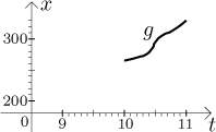
The standard notation for restriction is like this:
g = f |[10,11].
In words, by g we mean a function obtained by considering only the
part of f that corresponds to arguments from the interval
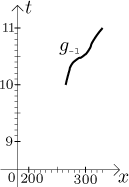
Since g is 1-1, we can find its inverse. For instance, from the graph we can guess
g(10) = 265, g(10.2) = 270, g(10.5) = 295 , g(10.8) = 315, g(11) = 330.
The inverse function therefore has values
g−1(265) = 10, g−1(270) = 10.2, g−1(295) = 10.5, g−1(315) = 10.8, g−1(330) = 11.
Since the inverse function takes as its arguments values of the original function, it follows that the domain of the inverse function is the same as the range of the function that is being inverted. Similarly, the range of the inverse function is arguments of the original one, that is, the domain of it. These two facts are true in general, here we have
The graph of the inverse function is obtained by exchanging the argument and value axes, that is, by flipping the picture about its main diagonal:
This concludes the survey of the most important properties of real functions.
Note on the inverse: In most textbooks, the inverse function is
denoted
Indeed, in our example, the inverse function
Now when we write
We will use this example again when we discuss the meaning of the derivative and again when we explain the Fundamental theorem of calculus.
We will now return to the beginning, to the problem of a moving car. We
started by saying that we were interested in how much distance we
travelled. We may consider this to be another function, d for
distance, and
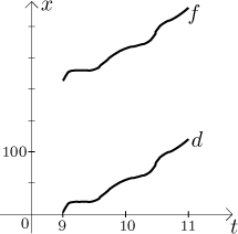
Thanks to this wonderful formula, knowing f we know d and vice
versa and all the relevant information is known. For instance, how much we
travelled between
Both functions d and f measured the movement itself. However,
often we have information about position rather than displacement. For
instance, we may imagine that the whole trip was on a fairly important road,
a road which has mile markers next to it. Assume that we started next to
the marker saying "17 mi" and stopped at the marker "134 mi". This
corresponds with the previous story, we did not turn back and the trip
took us 117 miles. Since we were only moving along the road, it means that we
are in a one-dimensional situation and the mile markers determine our
position precisely. In physics, the position at time t is usually
denoted
If we are only interested in how much we drove, then
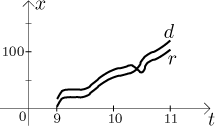
What happens if we for some reason double back? The mile markers recorded by our function will get smaller for a while, but we did drive some distance so d should increase! While odometer is not fooled, the position function stops being a direct source for our distance calculations. This shows that as long as we drive in one direction, the position and distance travelled are pretty much the same pieces of information, but in general they are not. Still, there is a way to recover the distance from the position. Common sense should suffice: Just identify the extremes of the journey (places where we changed directions) and by simple subtraction find how much was travelled between these turnaround points (between each two neighboring turning points we went in one direction only, so position gives distance). Those partial distances then can be added.
In general we need some more information, namely to relate the position and the displacement we need to know the derivative. By a remarkable coincidence, when we introduce the derivative in Derivative - Theory - Intro, we used just this example we now have to show how it relates to physics, in particular we showed that the derivative gives velocity. If you want to look at this note before you go further here, click here. So we will assume that we know about the derivative. We also used this example in this note, where we related the derivative and integral. What we argued there was that the distance we traveled can be recovered from the speed by the formula

The second equality follows from the fact that f and d
describe the same movement, they are just mutually shifted and therefore the
derivatives (velocities) they give must agree,

Similarly, the position function can be recovered from the velocity by the formula

But since speed is just the absolute value of velocity, which is the
derivative

Thus we found the relation between the position r and the displacement d.