Definition.
By a polynomial we understand any function of the form
p(x) = a0 + a1x + a2x2 +...+ anxn, where ak are real numbers.
Consider a polynomialp(x) = a0 + a1x + a2x2 +...+ anxn. We define the degree of p, denoteddeg(p), as the largest index k such thatak ≠ 0.
The fact that ak are real is sometimes emphasised by using the name "real polynomial". There are also other polynomials, for instance "complex polynomials" arise when we allow ak to be complex numbers. However, here we will only work with real functions, and so we just say "polynomials" and mean real polynomials.
The numbers ak are called coefficients. Some of them
may be zero, which means that the expression above is not unique for a given
polynomial. For instance, we can have
What is the degree of the zero polynomial (or constant zero function)? The
most popular choices are
We often use the phrase "let
The degree of polynomial satisfies the following properties:
(i)
(ii)
(iii) if
These formulas are definitely true for non-zero polynomials. Their general
validity dependas on how we define the degree of the zero polynomial.
If we set it to
In most situations it is enough to consider only polynomials with
The polynomial q is of the same degree as p and the most important properties of polynomials are the same for p and q, so it is often enough to investigate q (and it has the coefficient at the highest power equal to 1).
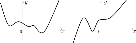
Shape of a polynomial.
For understanding polynomials it helps to know that when x gets close
to infinity (or negative infinity), then the leading term will win over the
other terms - they become unimportant. Thus a polynomial of degree n
has shape very similar to
These are the typical shapes for polynomials of even degree (on the left) and odd degree (on the right), assuming that there is a positive coefficient at the highest power.
If there is a negative coefficient (like in the polynomial
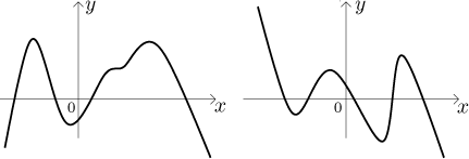
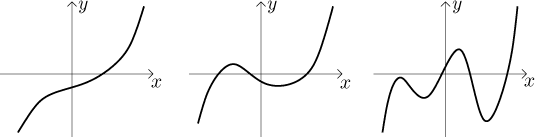
How many "bends" are there for a polynomial p? At most
From the typical shape it also follows that a polynomial of odd degree must have an even number of bends, since its "ends" at infinity and negative infinity always point in the opposite directions. On the other end, polynomials of even degree have "ends" pointing the same way, so they must have an odd number of bends. Thus for instance a polynomial of degree five can have these basic shapes:
Linear functions.
The name linear function denotes any function of the form
The angle at which the line goes up/down is given by the formula
The ability to quickly pass from a linear function to its graph and from a picture of a line to the formula that gives it is very useful, since linear functions belong among the most useful functions and appear very often.
Roots of a polynomial.
How many roots can we have for a non-zero polynomial p? Recall that by
a root we mean a number c such that
We see that it can have between 1 and 5 roots. In fact, polynomials of odd degree have always at least one real root.
Sidenote: The claim about number of roots would be true for all polynomials only if we decided that the zero polynomial has degree infinity, but that would play such a havoc with other properties that people do not do it.
In complex numbers, polynomials are better behaved. We will therefore briefly look at complex things, but we will quickly get back to reals. Note that real polynomials are also complex polynomials, since real numbers are a subset of complex numbers. Thus given a real polynomial, one can substitute complex numbers for x and pretend that it is a complex polynomial, drawing on some properties. We start right away with the main result.
Theorem.
Every polynomial (real or complex) of degree at least 1 has a complex root.Fact (factorization).
Let c be a root of a polynomial p. Then there is a polynomial q withdeg(q) = deg(p) − 1 such thatp(x) = (x − c)⋅q(x).
This Fact works in general for complex polynomials and complex roots, but if we start with a real polynomial and a real root, then the new polynomial q will be also real.
If we work in complex numbers, then we start with the Theorem, apply the Fact on factorization, and if the new polynomial q is not a constant, we can return to the Theorem and factor it further and so on, so we get
Corollary (factorization of polynomial to linear factors).
Letp(x) = anxn + an−1xn−1 +...+ a1x + a0 be a polynomial of degreen > 0. Then there are complex numbersc1,c2,...,cn which are all roots of p and satisfy
p(x) = an(x − c1)⋅(x − c2)⋅...⋅(x − cn).
Thus every non-zero polynomial has exactly as many complex roots as its degree (this also fits for degree zero), but some of these roots may be the same. When we put the corresponding roots together, we can rearrange the above decomposition into
Now di are distinct roots of p. Each corresponding power n(i) is called the multiplicity of the root di (see this note). For example, we may have
We would say that 1 is a root of multiplicity 2, while 3 is a root of multiplicity 1, also called a simple root.
Note that having such a nice decomposition with real coefficients is a matter of luck, since in general we are only guaranteed complex roots. Since we are only interested in real polynomials, we will now try to deduce some useful information that would not use complex numbers.
Fact.
If c is a complex root of a real polynomial p, then its complex conjugate is also a root of p.
This is wonderful, because it means that when we start factoring the
polynomials, for every term
Fact.
For a complex number c and its conjugate c* we have(x − c)⋅(x − c*) = x2 + ex + f, where e and f are real numbers.
Thus when we start with a real polynomial, we may get complex roots, but their factors can be put together in pairs to create real quadratic polynomials. Therefore we get
Corollary.
Every real polynomial can be written as
p(x) = an(x − d1)n(1)⋅...⋅(x − dN)n(N)⋅(x2 + e1x + f1)m(1)⋅...⋅(x2 + eMx + fM)m(M), where di, ej, and fj are real numbers.
In this decomposition, the linear terms
Such factorization can be very useful, and we see that having it is equivalent to knowing the roots of p. Unfortunately, finding such a factorization is generally next to impossible. Everybody and his dog knows the famous quadratic formula for finding roots of quadratic polynomials. There are also formulas for finding roots of cubic polynomials (degree 3), but they are not very pleasant and nobody remembers then anyway. Formulas for roots of polynomials of degree 4 are so ugly that most books actually skip them so as not to traumatize the more delicate reader. To top it off, one of major results of general algebra is that for polynomials of degree 5 and more there cannot exist any formula for roots.
Finding roots is thus a matter of chance and luck. Usually we try to guess
one root, then take out the corresponding factor
Example:
We try to factor
Solution: We see that
Thus we see that 0 is a root of p of multiplicity 3. What about
We obtained a quadratic polynomial, whose roots are 1 and −2 by the quadratic formula. Thus 1 is actually a root of multiplicity 2 and −2 is a simple root. We get
Note: Instead of using the quadratic formula, one can also try to guess the factorization, see this remark.
Example:
We try to factor
Solution: We try to guess, after a while we find that
The quadratic formula shows that
Example:
We try to factor
Solution: We try to substitute 0, 1, −1, 2, −2,..., but after a while we give up. What can we do? Since guessing did not help, this problem is not solvable by tools we know.
Note that the only irreducible polynomials are those of degree 1 (linear) and 2 (quadratic), so there must be some factorization of p. Perhaps there are real roots, but they are not integers so we can't guess them. Since the polynomial is of even degree, it might also happen that there are no real roots. In fact, that is exactly what is happening here, we have
How did we get it? We cheated, we created this example by starting with two irreducible quadratic polynomials and multiplied them together. If we did not know the answer from the very start, we would not know how to solve it.
Now we look at a different topic, related to factoring. We used the long
division of polynomials, in general one gets a remainder when dividing. To
show some motivation we recall the following: When we try to divide 17 by 5,
we get answer: It is 3, with remainder 2. We could write it as follows:
Remarkably, one can do the same for polynomials, instead of the magnitude of number we will use the degree of polynomial.
Fact (division with remainder).
Let p,q be polynomials. Then there are unique polynomials s,r such thatand
p(x) = s(x)⋅q(x) + r(x) deg(r) < deg(q).
Again, one can express it as
Sidenote: We have no restrictions on p and q in our theorem,
so one or both may be the zero polynomial. This fact remains true as long as
we define the degree of zero polynomial to be negative, so the popular
values
By a rational function we mean any ratio
Every rational function can be written as a sum of a polynomial and a proper rational function with the same denominator. This is just a reformulation of the Fact on division with remainder. In practice we do it using the algorithm for long division.
Since polynomials are relatively easy to handle, we see that in order to work with rational functions, in many situations it is enough to know how to work with proper rational functions. This is particular applies to the method of partial fractions decomposition. Since this method is very important, we dedicated a special section to it, and since the main use (at least for us) is for integration, we put that section there, so for partial fractions check out Integrals - Theory - Integration methods - Partial fractions.
Briefly, the method first calls for breaking the denominator q into linear and quadratic (if needed) factors as we discussed above, the proper rational function can be then broken into a sum of simple so-called partial fractions, very simple fractions whose denominators come from the linear and quadratic factors of q. A practical point of view is here.
One last note: When talking about polynomials we remarked that when x
is close to infinity (or negative infinity), then a polynomial is
essentially equal to its leading term. Therefore when
Exponentials, logarithms
Back to Theory - Elementary
functions