When we have a curve in the plane, whether given by a function or an implicit equation, we so far treated it as a shape. However, sometimes there is more information included in the situation, namely when the curve is actually a record of a movement, the path traced by, say, a bug.
The shape itself is not enough then, since two bugs can crawl along the same path in very much different ways (speed and even direction can vary, a bug can even turn back for a while and retrace the same path). This additional information has to be somehow stored and the most natural way is something called the parametric curve.
You obtain such a curve rather easily. At every time t that you are
interested in you record the position in plane, that is, the x and
y coordinate. Such a parametric curve is then described by two
functions depending on time,
Such a parametric description carries complete information including instantaneous velocity at every time. Given the general way in which a bug can move, the curve described by a parametric equation can be very complicated and there is little hope of describing it also as a graph of a function. However, we can attempt to describe at least parts of it using functions so that we can use the arsenal we already have at our disposal, above all our skills in graph sketching. But first we look at some examples.
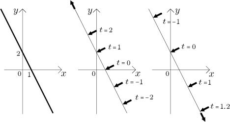
Example: Consider the parametric curve
What shape does this curve have? Here it is actually simple, since we can
eliminate the parameter t. From the first equation we get
Example: Consider the parametric curve
What shape does this curve have? Here it is not necessary to actually get
t itself from the first equation, we can write

but from the point of view of mathematics, when we investigate them as curves, they are the same.
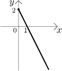
Example: Consider the parametric curve
We again have our straight line, but notice now that although t again
runs through all real numbers, we cannot get negative x. Thus this curve
is just the part of the straight line
Example: Consider the parametric curve
We do not know how it looks like, since we cannot express t from the first nor the second equation. To get some idea of the shape we would have to somehow use the methods from function sketching, but for than we need to know how to differentiate such curves. For another look at this example we refer to the section Parametric functions in Derivative - Methods Survey - Graphing.
When trying to treat parametric curves as functions we encounter the same trouble we had with implicit functions, namely that sometimes it is not possible since the curve has multiple values for the same x. We also adopt similar strategy. We are not attempting any total conversion, we settle for local description. Just like with implicit function, we have a theorem about being able to locally describe a "nice" parametric curve using a function.
Theorem.
Consider a parametric curve given byx = x(t), y = y(t) for t from some interval I. Let t0 be from the interior of I. Ifthen there exists a neighborhood U of (t0) ≠ 0,
x0 = x(t0) and a functiony = y(x) on U such thaty(t0) = y(x0) and there is a neighborhood J of t0 such that the set of points
{(x, y(x)) for x from U} is equal to the set of points
{(x(t), y(t)) for t from J}.
To see how this theorem is applied to the example above that we could not figure out, see Parametric functions in Derivative - Theory - Implicit and parametric functions. Again, this gives existence but does not help with actually finding the function. In practice we either use advanced graphing techniques or try to eliminate t as we did above. One such example is in Solved Problems.
Remarks:
1. The notation
2. When transforming a parametric curve into a function, we usually
try to do it piecewise. That is, we take the largest possible piece and try
to express it using a function, then we take a piece right next to it and try
to express it etc. The intervals that we use come naturally when we try to
solve one of the equations for t (usually the first one), since for
that we need injectivity. If J is a subinterval of I on which
The strategy therefore calls for splitting I into intervals on which
the function f (or
3. We talked about transforming parametric curves into functions. Does
it work the other way? When we have a graph of a function f, can we
express it as a parametric curve? The answer is definitely positive, it is
called parametrization of a curve and it is not unique, a given curve
can be expressed in infinitely many different ways. For instance, above we
had two parametric curves describing the same straight line, and we can
change the cube power in the second example to any other positive odd integer
power and get the same line again. In general, a graph of f for
x from an interval I can be naturally parametrized as
Bonus: Some famous curves.
Circle with radius r and center
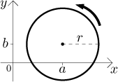
Note that the bug just goes around and around counterclockwise infinitely
many times, at a constant speed. Thus we get the same curve by changing the
bug's speed, for instance we can use
Ellipse with semi-major axis A, semi-minor axis
B, and center
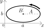
Note that the bug keeps going around counterclockwise, we can therefore restrict time as above.
Remark: Note that in the equation of the circle the parameter t actually tells us the angle with respect to the x-axis at which the bug is at any given time, the second info is the distance r from the center. We can play with this distance a bit, for instance we can make it depend on time as well.
Example: Consider this parametric curve:
If we try to substitute some prominent times (like
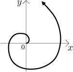
We obtained the Archimedes spiral. If we put a different function for radius, we can make other interesting shapes.
Remark: Note that t need not represent time. From mathematical point view we simply have some parameter (we may even use a different letter than t for it), the interpretation makes no difference. Moreover, in applications such a parameter may have an important meaning different from time, so once you understand parametric curves, it might be better not to get too hang up on the idea of time (especially since there are also parametric surfaces with more parameters, there the time idea falls through). However, the "time" point of view is so natural and above all helpful, that we decided to base our exposition of parametric curves on it. Of course, even if the parameter means something else, all methods covered here still work. And if you really run into trouble, you can at least pretend that the parameter is time and perhaps it helps (just don't tell anybody).