Problem: Sketch the graph of the function

Solution: We will use the procedure as outlined in Overview of graphing in Methods Survey - Graphing.

Step 1. The domain of this function is the whole real line, the function is continuous there. Since it is a polynomial with both even and odd powers, we suspect that it is not symmetric. We try one couple: For instance, f (1) = −9 while f (−1) = 13, which rules out the possibility that f is even or odd.

Before we proceed to intercepts, we need to get rid of the absolute value.

The x-intercept:

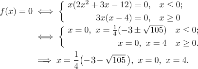
The two ugly roots in the first alternative are approximately −3.3 and 1.8, so we disregarded the latter, since that particular equation is relevant only for non-positive numbers. Note that f (0) = 0, so it also the y-intercept.

Step 2. We find limits at endpoints of the interval given by the domain.

Asymptotes: Since the function is continuous on the whole real line, there cannot be vertical asymptotes. Because limits at negative infinity and infinity diverge, there are no horizontal asymptotes there, but the limits exist and therefore there is a chance for oblique asymptotes. We will use the appropriate algorithm.

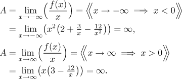
The limit for A diverged at both negative and positive infinity, therefore there are no oblique asymptotes there.

Step 3. We find the derivative and use it to determine monotonicity and local extrema. We will use the usual rules for every alternative, but note that they work only on open sets.

Critical points: There is one possible point in the domain where the derivative does not exist; we are not sure, but we need not decide for now, we will include x = 0 as a suspicious point where monotonicity can change. Where is the derivative zero?

The number x = 1 did solve the first equation, but for positive numbers that equation has nothing to do with f ′ and thus it was not a valid critical point. We have dividing points x = −2, x = 0, and x = 2. The domain thus splits into four intervals of monotonicity, we determine it using a table; we put closed endpoints when the function is continuous. We have to be careful and use every expression only in appropriate regions.

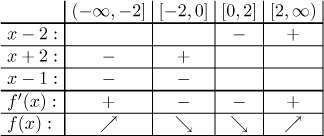
We have adjacent intervals of equal monotonicity, and since f is continuous at the connecting point 0, we know that they can be connected. The conclusion is that f is increasing on (−∞,−2] and on [2,∞) and decreasing on [−2,2].

Local extrema: The given function has a local maximum f (−2) = 20 and local minimum f (2) = −12. The point f (0) = 0 is not a local extreme.

We did not really need to know whether the derivative at 0 exists, so we skipped calculating one-sided derivatives, but their knowledge will help when we sketch the graph, so we include the calculation here to complete the part concerning the first derivative. We find them using a limit, see the appropriate theorem in Derivative and limit in Theory - MVT.

Surprisingly, there is a derivative at the connecting point, f ′(0) = −12. This means that the two parts of the graph connect smoothly, without a sharp bend.

Step 4. We find the second derivative and use it to determine concavity.

Dividing points: There is one point where the second derivative might not exist; since we do not really need to know, we save time by not exploring it and simply include x = 0 among dividing points. The second derivative is zero at x = −1/2, which is the second dividing point. The domain thus splits into three intervals of concavity, we determine it using a table; we put closed endpoints when the function is continuous.

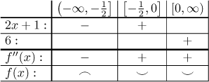
The conclusion is that f is concave down on (−∞,−1/2]; it is concave up on [−1/2,0] and on [0,∞).

Inflection points: There is one for sure, f (−1/2) = 6+1/2. It is not quite clear what is happening at zero. In fact, using limits and one-sided second derivatives one can show that there is even a second derivative at 0, f ′′(0)=6. Thus the function is actually concave up on [−1/2,∞).

Step 5. Now we put it all together. First we put all points and limit trends that we obtained above into a picture. This will be the skeleton on which we will hang the function. In order to save room we will change the scale on the y-axis.

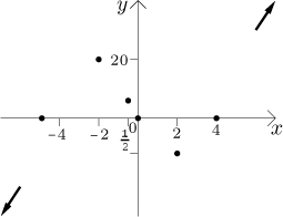
To see the shape of the graph better we combine the two tables above.

Now we are ready to sketch the graph.

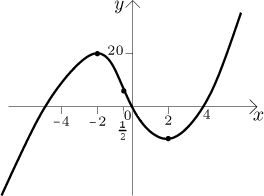
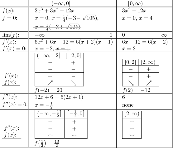
Remark: When working with functions given by cases, we split the real line into several regions according to its definition and then do the algorithm several times, in each region, and in each of them we disregard results that are outside that particular region. The above calculations can be (briefly) expressed like this.

Next problem
Back to Solved Problems - Graphing