Draining a tank

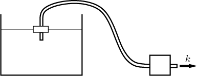
Here we will try to explore the following situation: We have a tank filled with water and we want to drain it. There are two natural quantities we can ask about: How much water was taken out of the tank and how much water is left in the tank. We will assume that draining started at time t = 0 and denote by V(t) the volume that was drained from the tank after time t since the draining started; by W(t) we denote the volume that is left in the tank at time t. We want to determine these two functions for each example of draining below.

Note that if we know how much water is there at the beginning, denote it V₀, then knowledge of one of the functions above automatically gives us also the second one, since they are connected by formulas

W(t) = V₀ − V(t),     V(t) = V₀ − W(t).

We will usually focus on V, the amount of water gone, since this is directly related to the mechanism in which the water is drained, therefore we expect easier formulas. Moreover, in case that V₀ is not known there is basically no way to determine W, while V can be (in most cases) found. Thus we have reasons to generally prefer V; however, under specific conditions W may be actually better to work with, see the last example.

Obviously, the answer (formulas for V and W) depends on how we do that draining. We will present three different ways of emptying the tank. The first one is trivial, but it shows some interesting ideas. The second example is the main one where we introduce all the important concepts of calculus. The third example probably looks simple, but in fact it is the hardest of all three and we would not be able to solve it without notions introduced in the second example. Before we start, one remark concerning units. They are irrelevant as long as we stick to the same units throughout our solution. For the sake of simplicity we will refer to liters and minutes here, you are welcome to substitute your own units for volume (gallons, cups, teaspoons, barrels, pints, six-packs, etc.) and time.

1. Pump with a constant action

Here we take a hose, stick one end into a pump and the other one into the tank (on a float if you wish) and start that pump. We will assume that the pump draws the water out at a certain steady rate k liters per minute.

This kind of problem is taught at elementary school. If we start draining at time 0, then at a certain time t the volume taken out is

V(t) = k⋅t.

(Assuming that t is not too large. After a certain time, namely V₀/k, there is no water left and this formula no longer applies, but then the situation is entirely trivial and not worthy our attention.)

And this is it, totally trivial, isn't it? We will now play with this simple situation, turning it this way and that way, it will all be really obvious so what's the point, well, we want to show some concepts and points of view that will come very handy later.

First, we also have a more general formula. The volume drained between times t₁ and t₂ is

k⋅(t₂ − t₁).

Second, the graph of V looks like this:

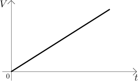
Where is the "drainage constant" k hidden in this picture? It is the slope of this line. If somebody gave us this graph, how would we recover this k from it? That is elementary, it is hidden in any right-angle triangle we care to draw next to this line with sides aligned by axes.

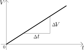
If we take a time interval somewhere on the x-axis, denote its size by Δt, and by ΔV we denote the corresponding output of water from the tank during this interval, then

This equation has some interesting features. If we insist that this equality must be true for all possible time intervals, then it determines the growth of V uniquely. However, it does not determine a function uniquely, because not just the function V above, but all its shifts have this growth; that is, all functions of the form Z(t) = k⋅t + a satisfy (1) for all time intervals. Thus we can actually use it for more general situations, when we do not start from zero but some water was drained in the past.

In more complicated situations we are often not able to supply a precise formula as the answer (the way we did above), but usually we are able to at least describe the desired function by some equations. The equation (1) is a good candidate, but it is not enough. As we observed above, it defines not one but a whole family of functions. If we want just one, we have to add another condition, and the previous paragraph hints at the natural one. We also need to specify what was the situation at the beginning, this is called an initial condition. In our case we start from zero. This should be enough; when we say where a function starts and how it should go from there, then it has no freedom of choice. Thus we arrive at a model of our situation.

The function V(t) is given uniquely by the following two conditions:
• V(0) = 0,   and
• the equation (1) is true for all time intervals Δt.

This is how a typical mathematical model looks like: Some equations such that if some function V satisfies them, then it describes our situation, and vice versa, the right function satisfies these equations. One important property of a model is uniqueness, meaning that only one function can satisfy it - we definitely would not like physics predicting that when we drop a stone, then it can either go down or fly up, depending how it feels at the moment. Our model does have it. Sometimes uniqueness is not possible by the nature of the situation we are studying, for instance when we drop a ball with its center of gravity going exactly at the edge of a knife, then nobody can guess which way it will tilt.

The above model has one interesting property: Its main part, that equation (1), is actually rather universal. It does not apply only to our example with the pump going at a steady rate. If a pump does all kinds of crazy things, then it settles down for a while and then again starts acting up, then the condition (1) still applies to all time intervals that lie in that part when the pump was going steady. This will be very useful below.

We tried to look at our simple situation from a more general standpoint and we will do another step in this direction. Let a function f (t) describe the rate at which the pump draws water at time t. Obviously this function is constant in our example, f (t) = k for all (relevant) t. What is the relationship between V and the graph of f ? The graph of f is a horizontal line at level k, and the above formula says that the value of V(t₀) is exactly the area under the graph of f on the interval [0,t₀].

More generally, water drawn between times t₁ and t₂ is equal to the area of the region under the graph of f over the interval [t₁,t₂].

Note that in that second, more general case that fact holds true whenever f is constant on the interval [t₁,t₂], its shape elsewhere does not play any role in it. This will come handy later.

As you can see, we got quite a bit out of this simple situation. Now we will see what happens with all these considerations when we pass to a more complicated situation.

2. Pump with a variable action

A real life pump does not work at a constant rate, because its action is influenced by many things, for instance the current supplied to its engine is never truly constant, the engine itself may exhibit some irregularities, etc. Moreover, you may influence its function yourself, for instance you may set it to run slower (and therefore quieter) at night or when your children sleep during the day. The rate at which it drains the water is therefore not a constant, but depends on time. As such it can be described by some function. For the purpose of this example we will assume that this rate (we will denote it by f ) is given by this graph, we chose something simple.

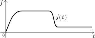
How can we interpret this? At the beginning we switched the pump on, but a real pump does not immediately jump to its peak performance, it goes there gradually. Then the pump ran at a (seemingly) constant rate for a while, then we lowered its draw (again, the change did not happen immediately).

Fine, we know how the pump pumped, what can we say about the function V describing the volume drained? One thing is clear, since f is not constant, we cannot use the previous procedure to get the whole answer. Is there any way to get at least some help from what we already know?

Here is an interesting idea. Take some time t₀ and consider a very tiny time segment around this particular time. Since f does not look too wild, we may assume that if we take a really really tiny segment, then f does not change almost at all on this segment, therefore we can assume that it is actually constant there without making a large error.

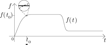
If we focus on that particular segment where we take f as a constant, we can apply the conclusions from the previous example (we discussed it there), in particular the graph of V is (on this segment) essentially a straight line with slope equal to f (t₀). Taking a hint from the first example, we can consider some triangle adjacent to that straight part of the graph of V with horizontal side of length Δt and the corresponding change in volume denoted by ΔV.

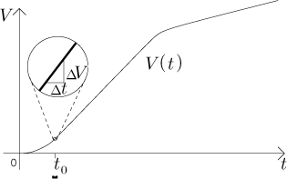
We only care about that little piece, so the shape of V elsewhere is irrelevant (which is good, since we do not know how V looks like yet). But it would look funny if we draw just a tiny piece hanging in the air, so we guessed the rest of V based on f: First the water drains slowly, but quickly the pump starts running and the drained volume grows fast; then we slow down the pump and the growth of V slows down accordingly. Anyway, as we said, we now look only at that little piece and from our guess that the graph of V is pretty much a straight line there we get

How do we get something precise about V from this "almost equality"? We know that f is almost but not quite constant on our segment, so we make some error there. We can also guess that the error we make gets smaller when we take smaller time segments. Thus the above "almost equality" gets closer and closer to equality when we take smaller and smaller time segments centered around t₀. The natural idea is to ask what would happen if we took infinitely many segments whose sizes decrease to 0. Intuitively one would expect that then the error goes to zero and the "almost equality" becomes equality. However, if we want to get something reliable, we have to explore this whole idea of working with infinitely many shrinking segments closer and find out how it behaves and what it does - and the notion of limit is born.

Assuming that we justified our idea of taking segments with sizes decreasing to zero, what happens on the left hand side of our (almost) equality? To see that we need to ask what that fraction actually means "in reality". Consider one such particular ratio ΔV/Δt. How does it read? The amount of water moved withing a certain the time segment divided by the size of this time segment. We know what this is, it is the average speed of water drainage. As we make the time segments home in on t₀, also the triangles are necessarily getting smaller and we are making average rates over smaller and smaller time intervals, so it is natural to expect that eventually we obtain the actual rate of drainage exactly at time t₀.

Thus when we start with the above "almost equation" and we do the shrinking procedure with segments and triangles, we get the following statement: The rate at which the water is drained at time t₀ is equal to the rate at which the pump is pumping then. Well, not exactly the discovery of the century, but it is nice to know that our reasoning yielded something that is obviously true, this suggests that we did not stray from the right path.

The important thing here is the way in which we arrived at this obvious statement, since it gives us an algorithm to determine that rate of change of V at time t₀, namely using approximating triangles. Being able to find the rate of change of some quantity is obviously a very useful thing when studying nature, since in nature everything changes and when we want to know what rules are behind it, the rate of change becomes crucial. Scientists therefore tried to explore the above algorithm of shrinking triangles theoretically, in a general setting, hoping to find general answers. They succeeded and discovered a simple algorithmic way in which we can deduce the rate of change for the given function. They decided to call this rate of change derivative, and use the notation V ′(t₀) for the rate of change of a function V at time t₀. Thus we can write the relation "discovered" above as V ′(t₀) = f (t₀).

This illustrates the point that mathematics is above all a language, here we used it to write precisely the "obvious" rule about rates of change. Only when we write it precisely, using mathematical notation, we can hope in deducing some information from it, for instance actually finding some formula for V.

The above equality should be true at every time, so it is a condition that forces V to grow in a certain way, at a certain rate. However, that does not describe the function V uniquely. We also have to say that at the beginning there was nothing drained. In this way we arrive at the model of our situation.

A function V describes how much water is drained from our tank if and only if this functions satisfies the following two conditions:
• V ′(t) = f (t) for all t,
• V(0) = 0.

When investigating some situation, creating the right model is usually the first and necessary step in the process of finding a solution. Trying to answer the question "What makes a certain thing change" usually turns into the following question: "What factors influence its rate of change?" Thus the notion of derivative appears naturally pretty much everywhere and modern science would not be possible without it.

Moral of the story, part 1: The derivative is a notion that appears naturally the moment you start asking good questions about the world around you (in fact physicists and mathematicians still argue about who came up with it first).

Now we will turn our attention to the main question: Can we actually find that function V determined by the above model?

We will again apply the idea that f is essentially constant on small segments, but now we do it globally. We start by fixing some segment size and then we divide the time axis into successive segments of this size. On each segment we replace f by its value in the middle of this segment.

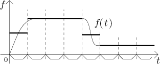
Now we will create a function V* that describes how much water would be drained assuming that the pump is described by the above piecewise-constant function instead of the real f. We start in the first segment, and if we denote its middle by t₁ then we assume that in that segment the pump pump goes at the constant speed f (t₁). Thus on this first segment V* should be a straight line with slope given by that constant rate of pumping. Then we get to the second segment. The pump goes at a steady rate there (this time given by the value of f at the middle point t₂), so the graph of V* must again be a straight line there, and since the amount of water drained cannot suddenly jump, the graph on the second segment must be connected with the graph from the first segment. In this way we continue and obtain something like the picture below (we scaled down the y-axis to get a picture of reasonable size).

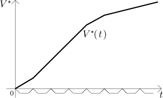
How faithful is this graph as an approximation of the real V? Let us compare what happens on the first segment. When we replace f by the middle value, then we at first overestimate the drainage, but on the second half we underestimate, so one could hope to argue that the difference is not all that large. However, this does not help with the second segment, where we consistently overshoot, which shows that this kind of argument is not really useful. A much better argument is this: We admit that the error of approximation may be large, but that is because we took huge segments. If we took very small segments, then the differences between f and the constants that we use would be much smaller, therefore the resulting V* should be a better guess for V.

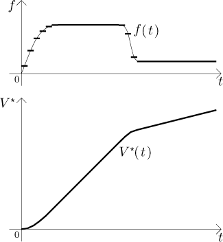
One might even hope that if we keep repeating this calculation with smaller and smaller segment size, then the graphs of the corresponding functions V* should approach the real graph of V. In fact, if f is not too wild (crazy oscillations cannot be approximated well by constants), then the above argument is true. The procedure we have just described is a starting point for two different directions of investigation, one practical and one theoretical.

From practical point of view it offers us an applicable way of approximating V(t₀) for some fixed t₀ by a formula that can be easily programmed into a computer. Indeed, the partial contribution of a pump drawing at a constant rate k over time segment of length Δt is k⋅Δt. When we divide the time interval [0,t₀] into small pieces, find the partial contribution of each and sum them up, we get

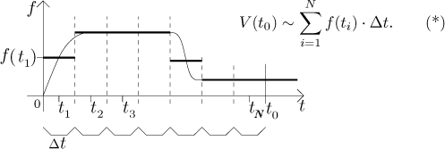
Of course, a very good question is how small the segments should be when we want to get the answer with a certain precision. There is a whole branch of mathematics that deals with such problems.

The theoretical view of that approximation by steps goes as follows. We can try to work out theoretically what happens when we repeat the above process infinitely many times with segment size decreasing to zero. Theory says that if f is reasonably nice, then indeed those graphs V* tend to V and in particular the summing formula above tends to a certain number A that is equal to V(t₀). Moreover, there exists a relatively reliable algebraic way of determining this number A. Does it have some meaning? We start by returning to the approximating formula (*) for V(t₀). In the first example we offered the following interpretation: This number is equal to the area of the region under the piecewise-constant function that replaced f in our calculations, on the interval [0,t₀].

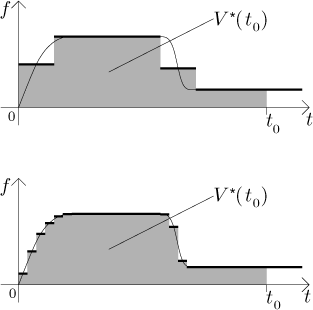
When we start making the rectangles more and more narrow, then the resulting piecewise-constant functions get closer and closer to f, so the number A that we get at the end is actually the area under the graph of f on the interval [0,t₀].

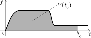
This number is called the definite integral of f from 0 to t₀ and we have a special notation for it, so we can rewrite the result that we obtained as

Recall that we have an algebraic way of finding this definite integral that works for nice functions quite reliably. This is what students learn in calculus courses.

Moral of the story, part 2: Integration is a way to sum up small contributions over time in case that these contributions are not constant, which again is something that one encounters quite frequently. The idea of integral appeared naturally when natural sciences were born. Thus we can put the blame on physicists, so it is definitely not true that mathematicians invented integrals in order to terrorize students.

Let us sum up what we did so far. We created a model of our situation, which was based on the equation V ′ = f, and then we have shown a way to solve this equation, that is, to find the function V that satisfies it. The main equation features the derivative of the unknown function, such equations are called differential equations. Most natural laws have this form. The one we have here is very simple. When differential equations get more complicated, we quickly find ourselves in a position that determining the solution by precise calculations is impossible. Then we turn to approximate methods and computers, in fact the algorithm with splitting into segments that we presented above is the basic method for numerical solving of differential equations.

Remark: We have an equation and we have a formula for its solution. What happens if we put them together?

We see that if we integrate and then differentiate, we get back to where we came from. Thus integration and differentiation are in a sense inverse procedures (almost but not exactly, we talk about it here in Math Tutor in section Fundamental Theorem of Calculus in Integrals - Theory - Introduction).

3. A hole in the tank

Now we use a different, but equally natural way to empty the tank, we pull the plug. Again, we want to determine the function V(t) describing how much water got out by the time t.

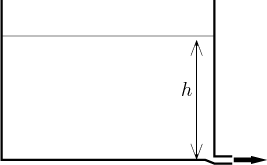
At what rate does the water pour out of the hole? First we will consider a very tiny time interval Δt that is so short that important parameters essentially do not change. We can imagine that the water that left the tank during this time formed a cylinder, its base is given by the hole and has the same area, call it a. The height of this cylinder is given by the velocity v of water (we may assume that it is constant during this very short time interval). When we start our time interval, some particle of water is at the hole (the cylinder has its base there), and by the time this interval stops, this particular particle of water traveled the distance v⋅Δt to form the top of the cylinder, so this number gives its height. Thus the volume ΔV that leaves the tank during this time is given by ΔV = a⋅v⋅Δt. This equation actually reads ΔV/Δt = a⋅v, so when we do the usual argument with making time intervals shorter and shorter, we obtain the following formula for the rate of change of V: V ′ = a⋅v.

The speed v depends on how much the water is pushed. They told us at elementary school that pressure in liquids does not depend on overall volume, but only on depth, that is, on the height of water column above this hole. We need to know the precise nature of this dependence and thus we turn to physics. Torricelli's law says that if the height of water column above the hole is h, then the speed is directly dependent on the square root of h. When we factor in the hole diameter and other factors (gravity, for instance) and hide them in one constant, we get a formula for the rate of change of V.

In order to make a reasonable equation out of it we need to get rid of h somehow. This means that we need to know more about our setup. The simplest relationship between volume and height of water happens when the tank has the same cross section at all levels (for instance when it is an upright cylinder or a rectangular box). If the area of this cross section is A (and we assume that the center of the hole is on the level with bottom), then we have the formula W = A⋅h, where W denotes the volume present in the tank.

We express h = W/A and substitute it into our equation, then we hide the constant A into k, it will become a different k but still a constant. Now we need to pass from W to V, for that we also need to know how much water there was initially, we denoted this V₀. Then we obtain the following equation:

This differential equation, coupled with the initial condition V(0) = 0, describes our situation. It is actually more complicated than it needs, we get a nicer formula if we focus not on water flowing out, but on water left. Recall that by W(t) we mean the volume of water that is left in the tank at time t. Given the mutual relationship between V and W, it is clear that the rate at which V grows is exactly the rate at which W decreases (so the sign of the derivative is minus) and vice versa. The above differential equation and initial condition then read

The minus is logical, the volume of water is decreasing, so the derivative (rate of change) must be negative. We derived a model that describes uniquely what is happening in the tank.

Note that this equation is fundamentally different from the one in the second example above. There we knew precisely right from the start how much water was drained at each individual moment, we just had to figure out some way of adding these individual contributions. Here we have a totally different situation. If we want to know how fast the water pours out right now, we would need to know how much water is there, but to know that we would need to know at what speed the water was pouring out at various times, but for that we would need to know how much water was there at those times, which we cannot know without knowing how fast the water was pouring out, and so on ad nauseam, it is a vicious circle.

Thus if we want to find a precise solution to this problem, we need to use more advanced methods. In fact, this problem is still quite simple as far as differential equations go, every student of calculus who heard of separation of variables should be able to deduce that W is necessarily given by this formula:

As usual, this formula only works until the tank is empty, it is easy to calculate the time when this happens.

We remarked above that when differential equations are too difficult to solve explicitly (giving the solution by formula as we did here), we turn to approximate calculations and computers. Out of curiosity, how would it work here?

We would fix a really tiny size of time segments Δt. The first segment of this size starts at the beginning, we may assume that throughout such a short time the volume and therefore the height of water column pretty much do not change. Thus the rate of outflow is essentially constant on this segment and it is equal to k times the root of V₀ (see the differential equation above); when we multiply this by the length of our time segment Δt, we obtain information how much water poured out during this short time segment. Then we subtract this small volume from the initial volume V₀, obtaining the number W₁, our approximation of the volume left at the end of the first time segment. This is the starting point for the second time segment.

We calculate new rate of change of volume using the above formula and the new volume W₁, and assume that this will stay that way throughout the second time segment, thus obtaining a constant flow there. Thus we can easily calculate how much water gets out and subtract it from W₁, obtaining W₂ - our best guess for the amount of water left at the end of the second time segment, which by the way is the time t = 2⋅Δt. The precise formulas are

We continue like this, drawing dots W_k that represent our approximations of W along the way, and when we connect them by straight segments, we get a graph that with a bit of luck is close to the actual graph of W. The procedure ends when we get to (or below) zero with the estimated volume. Repeating calculations like this is a piece of cake for a computer, and if we choose a really small size of the basic time segment, we get a pretty good approximation of the real solution given by the above formula.

Moral of the story, part 3: We have just shown how the first semester calculus can help in analyzing some fairly simple real-life situations, the second and the third problem could not be reasonably solved without it.

General note on models

The mathematical results that come out of a model fit the real situation only as well as the model describes it. This also applies to our examples. In the first two examples the underlying assumption was that the water that goes out of the tank is exactly the water that goes through the pump. Thus if our situation differs - the tank has a leak, the pump is not serviced well, the hose has a hole - and this difference is not negligible, then the theoretical formulas for V will not work.

Similarly, in the third example we assume that the hole we make is the only one, that the shape is regular as explained, and we also assume that the center of the hole is on the level with the bottom of the tank. Indeed, Torricelli's law uses h for the distance between the level the water reaches at a particular moment and the center of the hole. Thus is the hole is in some other place (for instance if we punch it a bit above the bottom), then the formula for h changes and we get a different equation and also a different solution.

Thus creating the right model has several stages. First we identify all factors that influence the process that we are studying. Then we try to capture in equations how that influence works. Next we attempt to solve this model, that is, to find function(s) that satisfy it. In case this is not possible (which is often), we use various numerical methods to obtain approximate solution(s). Then we have to ask how well this solution fits with the real situation we are studying, in particular how well does the model fit it. At this stage it gets really helpful if we can make a practical experiment (drain a concrete tank) and compare the observed values with those that we calculated here. If they agree, then this does not prove anything yet (we might have been just lucky), but it suggests that our work was not totally off. If they differ, we have to start looking for important influences that were missing in our model.

Next example
Back to Why?