Heat equation is one of the three basic partial differential equations. It describes how heat moves. We will use the knowledge of elementary first-semester calculus to guess this equation in a very simple setting.
Imagine that you have a steel bar. Initially it has some distribution of temperature, for instance we could have started our experiment by taking this bar out of a freezer and heating up one end very rapidly with flame. Then we stop the flame and look at what is the temperature of the bar at various places doing. The basic principle is that heat tends to move from places where there is lots of it to places where there is less.
We need to set up the situation first. For simplicity we will assume that
the bar is so thin that the temperature is always the same in its whole
cross section, so it changes only as we move along this bar. Thus in order to
describe the temperature of this bar, it is enough to take a function
We need one more simplifying assumption, we will assume that this bar does not exchange its heat with its surroundings, for instance because it is insulated. Also, we will not worry about its ends.
Now we are ready to start thinking about the right equation. As usual, the best starting point is to ask about change and what causes it. To this end, fix some time t and a position x on the bar. This is "our" place. We are interested in change of temperature in time at this place. At present we have some temperature, what would make "us" change it?
Since we assume no heat exchange with surroundings of the bar, the only relevant thing is the temperature of neighboring parts of this bar. Obviously, if the adjoint pieces to the left and to the right have the same temperature as "we" do, then we have no reason to change. Similarly, we have no reason for change if on one side the bar is warmer, but on the other side it is colder by exactly the same amount.
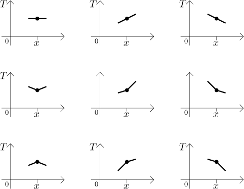
Thus we will change "our" temperature only if there is some imbalance between the adjoint parts of the bar. The greater the imbalance, the greater our change of temperature - this sounds logical. How do we express this mathematically? We get the right idea when we look at some pictures. We will now draw sample graphs of temperature along this bar at our time (we freeze the time for a moment). In the first row there are some examples of temperature distribution around us when we have no reason to change our temperature. In the second row there are examples when we want to increase our temperature, in the third row we want to decrease our temperature.

When you look at the shapes, you should immediately think of concavity. How do we find out about concavity of a function? We use the second derivative, here we need to differentiate twice with respect to the position on the bar, that is, with respect to x. How does it go? We want to increase our temperature (that is, the derivative of T with respect to time should be positive) if the function T taken just as a function of x is concave up, that is, when the second derivative of T with respect to x is positive. This shows direct dependence and we guess the following equation:
![]()
There is one serious problem with our conclusion. How did we know that the dependence is linear? What if the time derivative depends on, say, the third power of the second spatial derivative? Or perhaps some other dependence? That's where our guessing stops and serious physics starts (or experiments confirm that our guess was right on), the fact is that the above equation is correct. In more dimensions (when we work with volume instead of length and therefore we have more spatial coordinates x1, x2,...) it looks like this:

This heat equation is the basis for all situations involving temperature; things like no/partial/full insulation, outer sources of heat, various behaviour on the surface of the object and other factors just modify it, the core stays the same. There are thick books written about how to solve it in various situations, in more complicated settings we use numerical approximations on computers that share many common ideas with approximating tricks that we used in the previous section.
What was the point of this example? Well, if you looked at the pictures above and thought of concavity, then you experienced for yourself the main purpose of mathematics - to help in describing our ideas (and then with a bit of luck offer some solutions).