Functions of more variables: Local extrema

The usual definition of a local extreme carries over quite naturally to the case of more variables.

Definition.
Let f be a function defined on some neighborhood of a point ∈ℝⁿ.

We say that f has a local maximum at , or that f () is a local maximum, if there exists a neighborhood U = U() such that f () ≥ f () for all ∈U.

We say that f has a local minimum at , or that f () is a local minimum, if there exists a neighborhood U = U() such that f () ≤ f () for all ∈U.

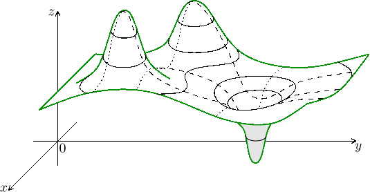
The picture below for the case of two variables shows two local maxima on the left and a local minimum on the right.

This is how we also imagine these notions for more dimensions. A local maximum has the property that if we slice the graph through that point in any direction (thus passing to the situation of one variable), then we still have a local maximum in the usual meaning on that slice. An analogous property is true for every local minimum.

In more dimensions there is a new kind of behaviour, we see it on the picture between the two hills. If we cut the graph there with a plane in direction leading between the hills, then we see a local maximum on the slice there in the valley. However, if we cut the graph using a perpendicular vertical plane (passing through the two summits), then in the valley we see a local minimum on the slice. Such points are called saddles or saddle points and we encounter them when investigating extrama, so they are usually counted among points to explore when a question asks about extrema.

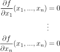
How do we find those local extrema? The procedure is similar to investigating local extrema for functions of one variable. Roughly speaking, first we find candidates using the first derivative, then we classify them using the second derivative.

If we cut the graph by an arbitrary vertical plane through some local extreme , we also get an extreme on the slice, so the derivative at in that direction must be equal to zero. If all directional derivatives are to be zero, then the gradient at (as a vector) must be zero as well.

Another reasoning: At a local extreme, the tangent plane must be horizontal, so its normal vector must be vertical. We observed in the previous chapter that for its normal vector we can take the vector

This vector is vertical exactly if () = 0 for all i, that is, ∇ f () = .

Theorem.
Let f be a function defined on some neighborhhood of a point ∈ℝⁿ. If f has a local extreme at and the gradient exists there, then ∇ f () = .

Points where ∇ f () = are called stationary points. With a bit of luck we can find them by solving the system of n equations () = 0 for n unknowns x₁,...,x_n.

As usual the statement does not work in the opposite direction, not every stationary point is a local extreme. Just recall saddle points that are stationary points but not extrema. So when we find stationary points, we need to classify them. For that we use the Sylvester criterion. It is easier to remember its conditions if you can imagine what is actually going on there.

A local maximum can be recognized by the fact that it is a maximum on all slices, in particular when cutting parallel to axes. In a one-variable situation we recognize a local maximum easily using the second derivative, so in case of more dimensions we expect a local maximum to satisfy () < 0 for all i. Similarly, for a local minimum we expect () > 0 for all i.

We now focus on the case of two variables. All extrema (maxima and minima) have one thing in common, the signs of (x, y) and (x, y) must agree, which we can express using the condition (x, y)⋅(x, y) > 0. Conversely, if (x, y)⋅(x, y) < 0, then the signs must differ, in one slice we see a maximum, in the other a minimum and we are obviously getting a saddle here.

We see that the product of non-mixed second derivatives can serve as a primary tool for telling apart saddles and extrema. And once we find that the point in question is an extreme, then to distinguish between a maximum and a minimum it is enough to check on some slice, that is, we just check on the sign of arbitrary non-mixed second derivative, for instance (x, y).

These observations were not completely wrong, but there is an unpleasant gap. We observed that an extreme has a positive product of the two second derivatives, but in fact the other direction is needed. If we find that the product is positive, does it mean that we have a local extreme? Unfortunately not.

The problem lies in the fact that we also have to take into account mixed derivatives, that is, we have to consider all entries of the Hess matrix

Above we used the product of its diagonal to make the first decision, perhaps it reminded the reader of determinant. It turns out that it indeed works this way, det(H) > 0 indicates an extreme, det(H) < 0 indicates a saddle. We obtain the following algorithm.

Investigating extrema for f (x, y).

1. By solving the equation ∇ f (x, y) = , that is, the system

we find stationary points .

2. For each stationary point we find the corresponding Hess matrix H = H().

3. If det(H) < 0, then there is a saddle at .

4. If det(H) > 0, then there is a local extreme at . It is a local maximum if () < 0, it is a local minimum if () > 0.

When zeros appear in key moments, then this algorithm fails, we know nothing and more advanced methods have to be used. That is a topic beyond this introduction.

If we want to generalize this procedure for more variables, we have to look at it from a different angle. First we notice that in step 4 we are actually also checking on a sign of some matrix, namely a submatrix of H given by its upper left corner. This is an interesting inspiration. We imagine a (large) matrix H and we ask what can be expected from its upper left subdeterminants of all sizes, these are traditionally denoted Δ_i. To avoid deeper theory we assume now that all mixed derivatives are zero, so H is a diagonal matrix, then determinant is just the product of the diagonal.

Recall that in case of a local maximum we expect () < 0 for all i, whereas in case of local minimum we expect () > 0 for all i.

• The first subdeterminant is the upper left entry of H, that is,

  

  It should be negative for maximum, positive for minimum.

• The second subdetermiant is given by the 2×2 matrix in the upper left corner of H, that is,

  

  It should be positive for both maximum and minimum.

• The third subdeterminant is given by the 3×3 matrix in the upper left corner of H, that is,

  

  It should be negative for maximum, positive for minimum.

You can surely work out how this should go on. For maxima the signs alternate, for minima all subdeterminants come up positive.

If there is some other progression of signs, then we do not have a maximum or minimum, and if some of the determinants are zero, then the whole procedure failed and we do not know what is going on at .

Our observations about a diagonal H are true in general.

Theorem (Sylvester criterion).
Let f be defined and have continuous second order partial derivatives on some neighborhood of a point that is stationary for f, that is, ∇ f () = 0. Let H be the Hess matrix of f at , let Δ_i be its upper left subdeterminants.

If Δ_i > 0 for all i, then f () is a local minimum.

If Δ₁ < 0, Δ₂ > 0, Δ₃ < 0, and so on up to (−1) ⁿΔ_n > 0, then f () is a local maximum.

Algorithm for investigating local extrema for f ().

1. By solving the equation ∇ f () = , that is, the system

we find stationary points .

2. For each stationary point we find the corresponding Hess matrix H = H().

3. We evaluate subdeterminants Δ_i, that is, determinants of upper left submatrices of size i×i.

4. If Δ_i > 0 for all i, then there is a local minimum at .
If the signs alternate Δ₁ < 0, Δ₂ > 0, Δ₃ < 0,..., then there is a local maximum at .

Example.
We find a classify local extrema of the function f (x, y,z) = 2xy² − 4xy + x² + z² − 2z.

First we find stationary points. The equation ∇ f () = is in this case

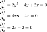
It is a system of three equations of three variables, this sounds hopeful, but the equations are not linear, so the whole nice theory is of no use. How do we solve general systems?

We start by noticing that the third equation is independent of the others, so definitely z = 1. What next? The most reliable method is by elimination, we keep expressing certain variables from equations and substituting them to others, thus reducing the number of equations and unknowns. Here we could use the first equation to find x = 2y − y² and substitute this into the second equation, creating an equation of third degree with unknown y, with a bit of luck this can be handled by smart factoring (try it). However, this looks a bit like an adventure, it is good to know some alternatives.

We focus on the second equation that we rewrite as 4x(y − 1) = 0. If we can create a product on one side and zero on the other, we hit the jackpot. In this particular case we see that there are two possibilities, x = 0 or y = 1.

The case y = 1 changes the first equation into −2 + 2x = 0, that is, x = 1 and we have the first stationary point (1,1,1).

The case x = 0 changes the first equation into y² − 2y = 0 and there are two solutions, y = 0 and y = 2. Thus we get two more stationary points, (0,0,1) and (0,2,1).

Now we have to investigate all three stationary points, so we need the Hess matrix. We prepare the second partial derivatives, thanks to the symmetry it is enough to calculate six of them:

The Hess matrix is

Here we go:

Point (1,1,1):

Signs go +, +, +, therefore f (1,1,1) = −2 is a local minimum.

Point (0,0,1):

Signs go +, -, -, therefore f (0,0,1) = −1 is not a local extreme.

Point (0,2,1):

Signs go +, +, -, therefore f (0,2,1) = 3 is not a local extreme.

Example.
We investigate local extrema of the function f (x, y) = xy e ^{x - y2/2}.

First we find stationary points.

Since the exponential is always positive, we can divide the equations by it and solve the equations (1 + x)y = 0 and x(1 − y²) = 0 instead. We rewrote the equations to the advantageous form of a product and the first one yields two possibilities.

If y = 0, then from the second equation we have x = 0. and the stationary point (0,0).

If x = −1, then from the second equation we have y = ±1. We found stationary points (−1,−1), (−1,1).

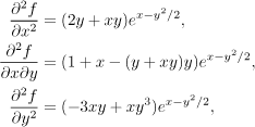
We prepare the second partial derivatives:

The Hess matrix is

Since we have a function of two variables, we use the first algorithm where we first check on Δ₂.

Point (0,0):

hence Δ₂ = −1 < 0 and f (0,0) = 0 is a saddle.

Point (−1,1):

hence Δ₂ = 2 > 0 and we have a local extreme. Since Δ₁ = 1 > 0, f (−1,1) = −e^−3/2 is a local minimum.

Point (−1,−1):

hence Δ₂ = 2 > 0 and we have a local extreme. Since Δ₁ = −1 < 0, f (−1,−1) = e^−3/2 is a local maximum.

Functions of more variables: Integral
Back to Extra - Functions of more variables