Overview of the NumericalMethods Package

Calling Sequence
    NumericalMethods[command](arguments)
    command(arguments)

Description

• The NumericalMethods package is a suite of commands that covers the following core topics of numerical analysis: integration, root finding, ODE solving, and working with matrices (solving systems of linear equations, finding eigenvalues and eigenvectors). The intended audience are students with little or no experience with Maple in a class whose purpose is not to teach Maple but to experiment with basic numerical methods. These commands are not meant to compete with corresponding commands from standard Maple libraries, but to supplement them in a specific setting.
  Advantages:
   - all these commands are available in one package;
   - they all share similar options (which agree with Maple's standard commands whenever possible and convenient),
   - they offer informative and intuitive output, which is not always the case with Maple's commands,
   - they allow for some experimentation not available with the usual Maple packages (e.g. choosing pivoting strategy for Gaussian elimination),
   - sometimes they offer more options (e.g. the option of specifying step size directly or by number of partition points).
  Disadvantages:
   - typically, these commands are less efficient and offer smaller range of methods than Maple's counterparts,
   - some of the commands lack descriptive graphical output (plots and animations for root finding and integration).
• Each command in the NumericalMethods package can be accessed by using either the long form or the short form of the command name in the command calling sequence. It is also possible to use the form NumericalMethods:-command.

List of NumericalMethods Package Commands

BackSubstitute        IntNumeric        MatrixEliminate        MatrixIterate        ODENumeric        ODENumericTaylor        PowerIterate        Root        SpectralRadius

Examples

> with(NumericalMethods):
> IntNumeric(sin(x), x=0..Pi, method=trapezoid, romberg=2, numsteps=21, output=information);
Using step size 0.149600.
Approximation of the integral by the chosen method with n=21 is  1.996268599.
Approximation of the integral by the chosen method with n=2*21 is  1.999067410.
The Romberg error estimate of the latter integral approximation is 0.000933.

> Root(exp(-x)-x, xinit=0, method=newton, tolerance=0.000001);
k=00  x=  0.0000000000   f(x)=  1.0000000000  test= 0.0000000000
k=01  x=  0.5000000000   f(x)=  0.1065306597  test= 0.5000000000
k=02  x=  0.5663110032   f(x)=  0.0013045098  test= 0.0663110032
k=03  x=  0.5671431650   f(x)=  0.0000001965  test= 0.0008321618
k=04  x=  0.5671432904   f(x)=  0.0000000000  test= 0.0000001254

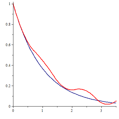
> ODENumericTaylor(diff(y(x),x,x)=-3*diff(y(x),x)-2*y(x), yinit=[1,-1], x=0..3.5, degree=2, stepsize=0.7, output=fullgraph,solution=exp(-x));

> MatrixEliminate(<<6,9>|<3,1>>, pivoting=euclidean);

> MatrixIterate(<<2,1>|<-1,3>>, <1,2>, xinit=<1.3,2.3>, method=gaussseidel, tolerance=0.001, stoppingcriterion=residual);
k=01  x=[  1.6500000000,  0.1166666667],   res= 2.1833333330   test= 2.1833333330,
k=02  x=[  0.5583333335,  0.4805555553],   res= 0.3638888883   test= 0.3638888883,
k=03  x=[  0.7402777775,  0.4199074073],   res= 0.0606481477   test= 0.0606481477,
k=04  x=[  0.7099537035,  0.4300154320],   res= 0.0101080250   test= 0.0101080250,
k=05  x=[  0.7150077160,  0.4283307613],   res= 0.0016846707   test= 0.0016846707,
k=06  x=[  0.7141653805,  0.4286115400],   res= 0.0002807790   test= 0.0002807790,

> PowerIterate(<<3,2>|<1,2>>, xinit=<1.3,2.3>, tolerance=0.001, matrix=[shift,3.5]);

Iterating with the matrix (A-3.5*E)
k=01  x=[  1.0000000000, -0.5151515152],    lambda= -1.9310595090
k=02  x=[  0.3661202185, -0.9999999998],    lambda= -2.3503344020
k=03  x=[  0.5299877603, -1.0000000000],    lambda= -2.5220075840
k=04  x=[  0.4941429595, -1.0000000000],    lambda= -2.4952372930
k=05  x=[  0.5011769229, -1.0000000000],    lambda= -2.5009384380
k=06  x=[  0.4997648367, -0.9999999998],    lambda= -2.4998117470
k=07  x=[  0.5000470415, -1.0000000000],    lambda= -2.5000376290