In some situations we do not get a function explicitly, but by an equation
that features both the unknown and the function. For instance, the equation
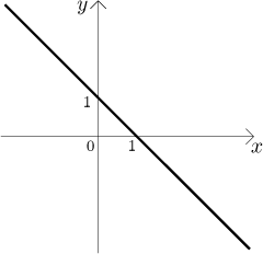
Example 1: Consider the equation
We used the known fact that equations of the form, say,
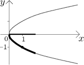
Example 2: Consider the equation
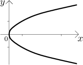
To see this we used a simple trick, we "switched" the variables and imagined
that x depends on y, then the equation describes the basic
parabola, we just have to draw it properly (with switched axes). Again, we
obtain a curve, but this time we cannot consider it a graph of some function.
On the other hand, we can make it up out of two graphs. Solving the equality
for y gives
![]() ,
,
Example 3: Consider the equation
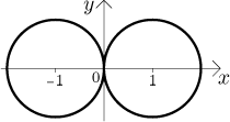
To see this we used another trick. If x was in the equation without the
absolute value, then the equation would describe a circle with radius 1 and
center
Example 4: Consider the equation
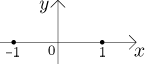
This example shows that an equation need not give a curve. Here we have two points, one can easily write an equation that describes even infinitely many points that are all isolated.
Example 5: Consider the equation
Example 6: Consider the equation
This example is quite interesting. When we try to solve the given equation for
y, we see that there are infinitely many solutions, functions
We used these examples to show that an equation can define very strange sets in the plane, so it would be naive to expect that we can always make a function out of it. To get a better insight we look closer at what is usually needed.
Problem: We have an equation with x and y. We also have
a point
Note that when investigating functions, we need some neighborhood to be able to find limits or a derivative, so it is natural to ask that we describe the curve as a function on a neighborhood of the given point.
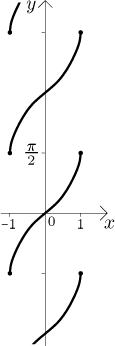
Back to Example 2: If somebody gives us a point ![]() ,
,
In other words, locally, on a neighborhood of the given point, we were able to
solve the given equation for y.
Similarly, if somebody gives us a point ![]() ,
,
Thus we can again locally express the curve as a function, but a different
function then before. This is quite normal. Finally, consider the point
This tells us the following. If we have a curve given by an equation, we often have a chance to express its parts around given points by functions (implicit functions), but sometimes this is not possible. Is there a way to somehow tell "good" points from "bad" points? In fact, there is, but it requires more advanced math (functions of more variables, partial derivatives). We will include the relevant statement here for the sake of completeness.
Theorem (Implicit function theorem).
Consider an equationF(x, y) = c. Let a point(x0, y0) satisfy this equation. If
then there exists a neighborhood U of x0 and a function
y = y(x) on this neighborhood such thaty(x0) = y0 andF(x, y(x)) = c for all x from U.
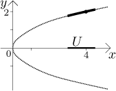
Example: Consider the curve given by
Solution: First we rearrange this equation to fit the above pattern:
Now we find the necessary partial derivative.
![]()
Since this derivative is not zero, by the Implicit function theorem there is
a desired function on some neighborhood of
What good is then all this business? First, we see that implicit curves are a richer family then the family of possible "nice" graphs of functions. In other words, we can easily describe implicitely objects that would be rather difficult to trace using graphs of functions (see below). That's the advantage of implicitly defined curves.
On the other hand, when we want to investigate these curves (for instance find tangent lines), we would much prefer to treat them as functions, since then we have very powerful tools. The theorem above tells us something, perhaps not too much, but note that tangent lines just happens to be a problem where local knowledge close to a given point is enough. What is even more interesting, there is a way to find derivative of an implicit function without really knowing its formula, just using the equation that defines it. This can be quite useful, see Implicit differentiation in Derivative - Theory - Implicit and parametric functions.
Two examples of working with implicit functions on the level we know now can be found in Solved Problems.
One last remark: We talked about changing implicit curves into functions. Can
it be done the other way? The answer is positive and it is so simple that we
are not going to waste another paragraph on it. If a curve is given as a
graph of some function
Bonus: Some famous curves.
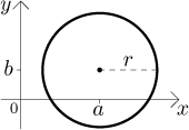
Circle with radius r and center
Ellipse with semi-major axis A, semi-minor axis
B, and center
![]()
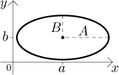
Obviously, taking
Parametric functions
Back to Theory - Implicit and
parametric functions