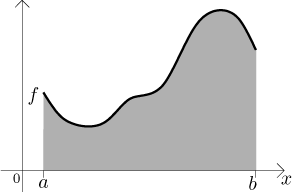
Motivation: Consider a function f defined on a closed interval
If we can somehow determine the area of this region, we will call this number the definite integral of f from a to b.
There are many ways to try to determine the area. Depending on the properties of the function f, it may be difficult or even impossible to do so. Here we will try the approach of Riemann. It is based on a simple observation that the area of a rectangle is easy to calculate. Therefore we try to approximate the region under the graph of f by suitable rectangles.
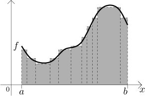
It seems from the picture that if we made the rectangles really narrow, the error of approximation would be small. By taking narrower and narrower rectangles, with a little bit of luck the resulting approximated areas converge to some number, namely the area of the region under the graph of f. This procedure can break down if the approximation errors do not get smaller for narrower rectangles; this depends on the shape of f, for really wild functions the region is strange and it may not make any sense to talk about its area.
Now we will make this procedure precise.
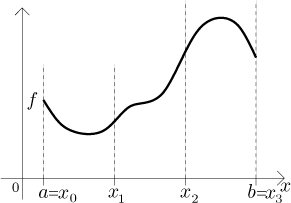
The widths of rectangles are determined by splitting the interval
Definition.
Consider a closed interval[a,b]. By a partition of[a,b] we mean any finite setP={x0, x1,..., xN} of points from[a,b] such thata = x0 < x1 < . . . < xN = b.
Assume that we have a bounded function f on an interval
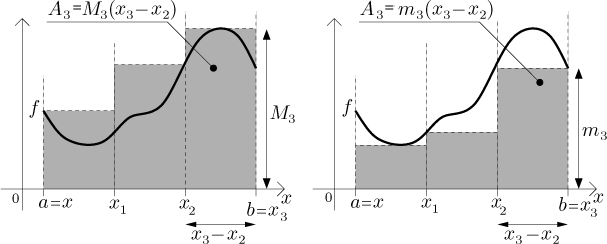
Now we have to decide on their heights. There are several methods, here we use the one that is easiest to handle. To be on the safe side, we look at the largest and smallest possible (and reasonable) rectangles, obtaining the upper sum and the lower sum:
Definition.
Let f be a bounded function defined on a closed interval[a,b]. Given a partition P of[a,b], fork = 1,...,N, set
We define the upper sum associated with P by
We also define the lower sum associated with P by
Note that since the function f is bounded, the suprema and infima in the definition always exist finite. Therefore the sums make sense. In both sums we are adding areas of rectangles. Their bases are given by the partition, the heights by the supremum or infimum of f in each rectangle.
The upper and lower sum is shown in the following pictures. On the left, the area of the shaded region is the upper sum; on the right, the area of the shaded region is the lower sum. We also indicated expressions connected with calculating the area of the third rectangle.
If we denote the area under the graph of f by A (hoping that it makes sense), then from the picture it seems clear that
![]()
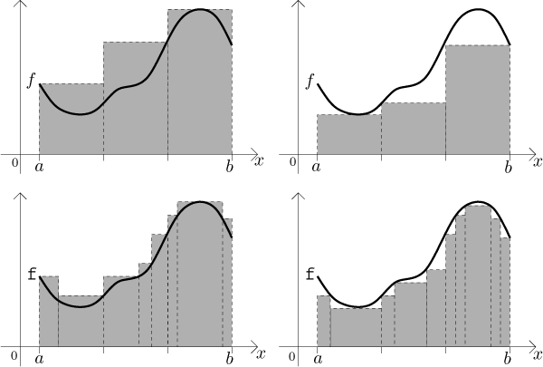
To determine the area A we will try to manipulate the rectangles so that the upper sum gets smaller and the lower sum gets larger, until they get almost equal. Since the area is always between the upper and lower sum, equality between the two sums means that we determined A. This manipulation has the form of taking narrower rectangles. The error of approximation is then smaller, which means that the upper sum gets smaller (and therefore closer to A) and the lower sum gets larger (and closer to A). In the next picture, compare the error of approximation of the upper and lower sum when we refine the partition.
The advantage of the upper/lower sum approach is that we do not have to worry about mechanics of this procedure, all the details are hidden in the definition below. Unfortunately, the Riemann approach using rectangles succeeds only if the function f is nice enough, when f is Riemann integrable. Precisely:
Definition
Let f be a bounded function defined on a closed interval[a,b]. We say that f is Riemann integrable on[a,b] if the infimum of upper sums through all partitions of[a,b] is equal to the supremum of all lower sums through all partitions of[a,b]. Then we define the Riemann definite integral of f from a to b by
We usually just say Riemann integral, it is understood that we mean the definite integral. Since for Riemann integrable functions, the infimum of upper sums is equal to the supremum of lower sums, we could also use the latter to determine the Riemann integral.
The snaky shape is called the integration sign, it is in fact a very
elongated S (for sum). The integrated function is sometimes called the
integrand. We have the lower limit a and the upper
limit b, giving the integrating interval
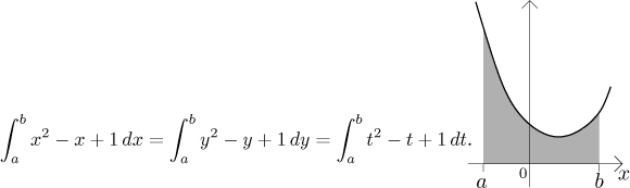
Indeed, the area under the same piece of the given parabola is always the same, regardless of what letter we write next to the horizontal axis.
For a more thorough explanation of the meaning of the integral notation (not mathematically correct, but very useful for understanding the concept), click here.
In our definition, we put the smaller limit (the left endpoint) as a lower
limit. Sometimes we may want to "integrate backward", from b to
a. Often we want to be able to simply write the integral without
worrying about the order, so we need a more general definition. This
is done as follows: Let
![]()
Now that we can integrate with any order of limits, the above equation becomes a general rule: We can switch the limits in the integral, provided we also add the minus sign in front.
Example: We investigate the integral
![]()
We need to decide on some partitions that would involve smaller and smaller
segments, hoping that the corresponding upper and lower sums will get closer
until they agree. Unless there is a good reason to do otherwise, it is
usually a good idea to try a regular partition, that is, given a natural
number N, split the interval
![]()
Now we need to determine the suprema and infima for the sums, but this should be easy just by looking at a picture:
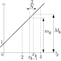
We can calculate the upper and lower sum:
Since our partitions are very specific, one can not expect that in general they would already give us the area (in the definition, we investigated all possible partitions). However, here the function is very nice and it turns out that when we send N to infinity, the sums approximate the area well. We have to be a little bit more careful to do it properly by definition:
Thus
![]()
that is,
![]()
Hence the function
![]()
We can check that this answer is correct by direct calculation from the picture using the formula for the area of a trapezoid.
The above calculation was not easy, even though we were lucky that we remembered the formula for adding first N natural numbers. For more complicated functions, it may be impossible to determine an explicit formula for the upper and lower sums. This is the reason why we usually use other means than the definition for evaluating Riemann integrals (see The Fundamental Theorem of Calculus).
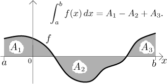
In our pictures we always had a positive function; the Riemann integral is then equal to the geometric area of the region between the graph of f and the x-axis. What if we have a negative function? Since the value of f determines the height of rectangles, we get areas with negative sign. Therefore, for negative functions, the Riemann integral is equal to minus the geometric area of the region between the graph of f and the x-axis.
For a general function, the Riemann integral is equal to the mathematical area of the region between the graph of f and the x-axis, that is, the geometric area of the parts above the x-axis minus the geometric area of the parts below the x-axis. For instance, in the following picture, A with subscripts 1,2,3 denote geometric areas of the individual parts:
This is a very important question. For our purposes, the most useful fact is this:
Theorem.
Every continuous function on a closed interval is Riemann integrable on this interval.
This example shows that if a function has a point of jump discontinuity, it may still be Riemann integrable. On the other hand, the example of Dirichlet function shows that if there is too many points of discontinuity, the function is not Riemann integrable. In fact, a function defined on a closed interval is Riemann integrable there exactly if it does not have too many points of discontinuity. For more information, click here.
The fact that Riemann integrability is not hurt by a finite number of
discontinuities is related to the fact that the value of Riemann integral is
not influenced by a change of the integrated function at a finite number of
points. Precisely, assume that f is Riemann integrable on an interval
To see why this could be true, look at the following picture, where we obtained g by adding 1 to the function f at the point c.
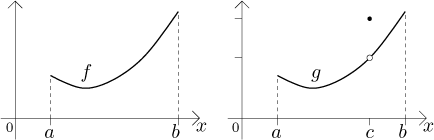
The region under the graph of g is the same as the region under the graph of f, plus an extra vertical segment at the point where we changed f into g. Since this segment has the thickness of one point, which is zero, its area is also zero and therefore there is no extra area under g.
We will close this section with one useful statement:
Theorem.
Every monotone function on a closed interval is Riemann integrable on this interval.
Properties of the Riemann integral
Back to Theory - Introduction